pacman::p_load(knitr, spdep, tmap, sf,
ggpubr, GGally, funModeling,
corrplot, GWmodel,
tidyverse, blorr, skimr, caret)In Class Exercise Week 5 - Investigation of functional and non functional water points using Geographical Weighted Logistic Regression (GWLR) in Nigeria
Overview
Water is a crucial resource for humanity. People must have access to clean water in order to be healthy. It promotes a healthy environment, peace and security, and a sustainable economy. However, more than 40% of the world’s population lacks access to enough clean water. According to UN-Water, 1.8 billion people would live in places with a complete water shortage by 2025. One of the many areas that the water problem gravely threatens is food security. Agriculture uses over 70% of the freshwater that is present on Earth.
The severe water shortages and water quality issues are seen in underdeveloped countries. Up to 80% of infections in developing nations are attributed to inadequate water and sanitation infrastructure.
Despite technological advancement, providing rural people with clean water continues to be a key development concern in many countries around the world, especially in those on the continent of Africa.
We will attempt to conduct logistic regression of the Osun state in Nigeria with the water points attributes in this exercise.
Getting Started
First, we load the required packages in R
Spatial data handling & Clustering
- sf, spdep
Choropleth mapping
- tmap
Attribute data handling
- tidyverse especially readr, ggplot2 and dplyr and funModeling
Exploration Data visualization and analysis
- corrplot, ggpubr, GGally, knitr and skimr
Logistic Regression
- blorr, caret, GWModel
Spatial Data
First we load the Osun spatial features using readRDS()
osun = readRDS("data/rds/Osun.rds")
st_crs(osun)Coordinate Reference System:
User input: EPSG:26392
wkt:
PROJCRS["Minna / Nigeria Mid Belt",
BASEGEOGCRS["Minna",
DATUM["Minna",
ELLIPSOID["Clarke 1880 (RGS)",6378249.145,293.465,
LENGTHUNIT["metre",1]]],
PRIMEM["Greenwich",0,
ANGLEUNIT["degree",0.0174532925199433]],
ID["EPSG",4263]],
CONVERSION["Nigeria Mid Belt",
METHOD["Transverse Mercator",
ID["EPSG",9807]],
PARAMETER["Latitude of natural origin",4,
ANGLEUNIT["degree",0.0174532925199433],
ID["EPSG",8801]],
PARAMETER["Longitude of natural origin",8.5,
ANGLEUNIT["degree",0.0174532925199433],
ID["EPSG",8802]],
PARAMETER["Scale factor at natural origin",0.99975,
SCALEUNIT["unity",1],
ID["EPSG",8805]],
PARAMETER["False easting",670553.98,
LENGTHUNIT["metre",1],
ID["EPSG",8806]],
PARAMETER["False northing",0,
LENGTHUNIT["metre",1],
ID["EPSG",8807]]],
CS[Cartesian,2],
AXIS["(E)",east,
ORDER[1],
LENGTHUNIT["metre",1]],
AXIS["(N)",north,
ORDER[2],
LENGTHUNIT["metre",1]],
USAGE[
SCOPE["Engineering survey, topographic mapping."],
AREA["Nigeria between 6°30'E and 10°30'E, onshore and offshore shelf."],
BBOX[3.57,6.5,13.53,10.51]],
ID["EPSG",26392]]Aspatial Data
Next we load the Osun water point data using readRDS()
osun_wpt_sf = readRDS("data/rds/Osun_wp_sf.rds")
freq(data=osun_wpt_sf, input = 'status')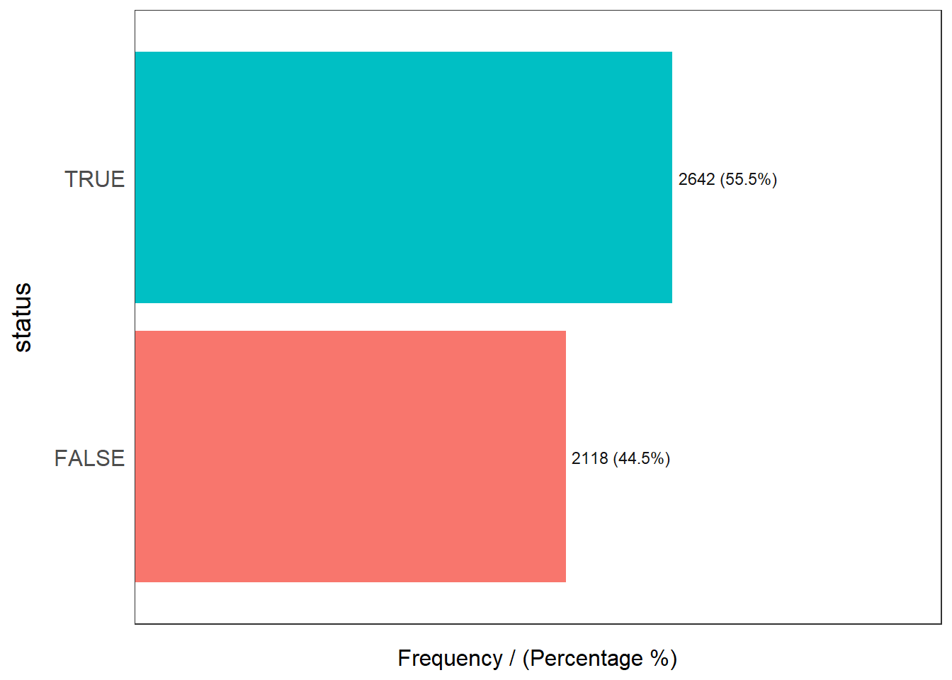
status frequency percentage cumulative_perc
1 TRUE 2642 55.5 55.5
2 FALSE 2118 44.5 100.0We can see that 55.5% of the water points are functional and 44.5% of the rest are not.
We toggle the mode to interactive mode by using ttm() and plot the map using functions from the tmap package of the status of the water points
ttm()
tm_shape(osun) +
tm_polygons(alpha = 0.4) +
tm_shape(osun_wpt_sf) +
tm_dots(col="status")Exploratory Data Analysis
Using the skimr package, we can give a brief summary statistics of the variables found in the osun_wpt_sf data frame. This can help us determine which variables we can choose by looking at the data completion rate. If data completion rate for a particular variable is poor, we will not want to use it or it can potentially present analysis that is inaccurate.
osun_wpt_sf %>%
skim()| Name | Piped data |
| Number of rows | 4760 |
| Number of columns | 75 |
| _______________________ | |
| Column type frequency: | |
| character | 47 |
| logical | 5 |
| numeric | 23 |
| ________________________ | |
| Group variables | None |
Variable type: character
| skim_variable | n_missing | complete_rate | min | max | empty | n_unique | whitespace |
|---|---|---|---|---|---|---|---|
| source | 0 | 1.00 | 5 | 44 | 0 | 2 | 0 |
| report_date | 0 | 1.00 | 22 | 22 | 0 | 42 | 0 |
| status_id | 0 | 1.00 | 2 | 7 | 0 | 3 | 0 |
| water_source_clean | 0 | 1.00 | 8 | 22 | 0 | 3 | 0 |
| water_source_category | 0 | 1.00 | 4 | 6 | 0 | 2 | 0 |
| water_tech_clean | 24 | 0.99 | 9 | 23 | 0 | 3 | 0 |
| water_tech_category | 24 | 0.99 | 9 | 15 | 0 | 2 | 0 |
| facility_type | 0 | 1.00 | 8 | 8 | 0 | 1 | 0 |
| clean_country_name | 0 | 1.00 | 7 | 7 | 0 | 1 | 0 |
| clean_adm1 | 0 | 1.00 | 3 | 5 | 0 | 5 | 0 |
| clean_adm2 | 0 | 1.00 | 3 | 14 | 0 | 35 | 0 |
| clean_adm3 | 4760 | 0.00 | NA | NA | 0 | 0 | 0 |
| clean_adm4 | 4760 | 0.00 | NA | NA | 0 | 0 | 0 |
| installer | 4760 | 0.00 | NA | NA | 0 | 0 | 0 |
| management_clean | 1573 | 0.67 | 5 | 37 | 0 | 7 | 0 |
| status_clean | 0 | 1.00 | 9 | 32 | 0 | 7 | 0 |
| pay | 0 | 1.00 | 2 | 39 | 0 | 7 | 0 |
| fecal_coliform_presence | 4760 | 0.00 | NA | NA | 0 | 0 | 0 |
| subjective_quality | 0 | 1.00 | 18 | 20 | 0 | 4 | 0 |
| activity_id | 4757 | 0.00 | 36 | 36 | 0 | 3 | 0 |
| scheme_id | 4760 | 0.00 | NA | NA | 0 | 0 | 0 |
| wpdx_id | 0 | 1.00 | 12 | 12 | 0 | 4760 | 0 |
| notes | 0 | 1.00 | 2 | 96 | 0 | 3502 | 0 |
| orig_lnk | 4757 | 0.00 | 84 | 84 | 0 | 1 | 0 |
| photo_lnk | 41 | 0.99 | 84 | 84 | 0 | 4719 | 0 |
| country_id | 0 | 1.00 | 2 | 2 | 0 | 1 | 0 |
| data_lnk | 0 | 1.00 | 79 | 96 | 0 | 2 | 0 |
| water_point_history | 0 | 1.00 | 142 | 834 | 0 | 4750 | 0 |
| clean_country_id | 0 | 1.00 | 3 | 3 | 0 | 1 | 0 |
| country_name | 0 | 1.00 | 7 | 7 | 0 | 1 | 0 |
| water_source | 0 | 1.00 | 8 | 30 | 0 | 4 | 0 |
| water_tech | 0 | 1.00 | 5 | 37 | 0 | 20 | 0 |
| adm2 | 0 | 1.00 | 3 | 14 | 0 | 33 | 0 |
| adm3 | 4760 | 0.00 | NA | NA | 0 | 0 | 0 |
| management | 1573 | 0.67 | 5 | 47 | 0 | 7 | 0 |
| adm1 | 0 | 1.00 | 4 | 5 | 0 | 4 | 0 |
| New Georeferenced Column | 0 | 1.00 | 16 | 35 | 0 | 4760 | 0 |
| lat_lon_deg | 0 | 1.00 | 13 | 32 | 0 | 4760 | 0 |
| public_data_source | 0 | 1.00 | 84 | 102 | 0 | 2 | 0 |
| converted | 0 | 1.00 | 53 | 53 | 0 | 1 | 0 |
| created_timestamp | 0 | 1.00 | 22 | 22 | 0 | 2 | 0 |
| updated_timestamp | 0 | 1.00 | 22 | 22 | 0 | 2 | 0 |
| Geometry | 0 | 1.00 | 33 | 37 | 0 | 4760 | 0 |
| ADM2_EN | 0 | 1.00 | 3 | 14 | 0 | 30 | 0 |
| ADM2_PCODE | 0 | 1.00 | 8 | 8 | 0 | 30 | 0 |
| ADM1_EN | 0 | 1.00 | 4 | 4 | 0 | 1 | 0 |
| ADM1_PCODE | 0 | 1.00 | 5 | 5 | 0 | 1 | 0 |
Variable type: logical
| skim_variable | n_missing | complete_rate | mean | count |
|---|---|---|---|---|
| rehab_year | 4760 | 0 | NaN | : |
| rehabilitator | 4760 | 0 | NaN | : |
| is_urban | 0 | 1 | 0.39 | FAL: 2884, TRU: 1876 |
| latest_record | 0 | 1 | 1.00 | TRU: 4760 |
| status | 0 | 1 | 0.56 | TRU: 2642, FAL: 2118 |
Variable type: numeric
| skim_variable | n_missing | complete_rate | mean | sd | p0 | p25 | p50 | p75 | p100 | hist |
|---|---|---|---|---|---|---|---|---|---|---|
| row_id | 0 | 1.00 | 68550.48 | 10216.94 | 49601.00 | 66874.75 | 68244.50 | 69562.25 | 471319.00 | ▇▁▁▁▁ |
| lat_deg | 0 | 1.00 | 7.68 | 0.22 | 7.06 | 7.51 | 7.71 | 7.88 | 8.06 | ▁▂▇▇▇ |
| lon_deg | 0 | 1.00 | 4.54 | 0.21 | 4.08 | 4.36 | 4.56 | 4.71 | 5.06 | ▃▆▇▇▂ |
| install_year | 1144 | 0.76 | 2008.63 | 6.04 | 1917.00 | 2006.00 | 2010.00 | 2013.00 | 2015.00 | ▁▁▁▁▇ |
| fecal_coliform_value | 4760 | 0.00 | NaN | NA | NA | NA | NA | NA | NA | |
| distance_to_primary_road | 0 | 1.00 | 5021.53 | 5648.34 | 0.01 | 719.36 | 2972.78 | 7314.73 | 26909.86 | ▇▂▁▁▁ |
| distance_to_secondary_road | 0 | 1.00 | 3750.47 | 3938.63 | 0.15 | 460.90 | 2554.25 | 5791.94 | 19559.48 | ▇▃▁▁▁ |
| distance_to_tertiary_road | 0 | 1.00 | 1259.28 | 1680.04 | 0.02 | 121.25 | 521.77 | 1834.42 | 10966.27 | ▇▂▁▁▁ |
| distance_to_city | 0 | 1.00 | 16663.99 | 10960.82 | 53.05 | 7930.75 | 15030.41 | 24255.75 | 47934.34 | ▇▇▆▃▁ |
| distance_to_town | 0 | 1.00 | 16726.59 | 12452.65 | 30.00 | 6876.92 | 12204.53 | 27739.46 | 44020.64 | ▇▅▃▃▂ |
| rehab_priority | 2654 | 0.44 | 489.33 | 1658.81 | 0.00 | 7.00 | 91.50 | 376.25 | 29697.00 | ▇▁▁▁▁ |
| water_point_population | 4 | 1.00 | 513.58 | 1458.92 | 0.00 | 14.00 | 119.00 | 433.25 | 29697.00 | ▇▁▁▁▁ |
| local_population_1km | 4 | 1.00 | 2727.16 | 4189.46 | 0.00 | 176.00 | 1032.00 | 3717.00 | 36118.00 | ▇▁▁▁▁ |
| crucialness_score | 798 | 0.83 | 0.26 | 0.28 | 0.00 | 0.07 | 0.15 | 0.35 | 1.00 | ▇▃▁▁▁ |
| pressure_score | 798 | 0.83 | 1.46 | 4.16 | 0.00 | 0.12 | 0.41 | 1.24 | 93.69 | ▇▁▁▁▁ |
| usage_capacity | 0 | 1.00 | 560.74 | 338.46 | 300.00 | 300.00 | 300.00 | 1000.00 | 1000.00 | ▇▁▁▁▅ |
| days_since_report | 0 | 1.00 | 2692.69 | 41.92 | 1483.00 | 2688.00 | 2693.00 | 2700.00 | 4645.00 | ▁▇▁▁▁ |
| staleness_score | 0 | 1.00 | 42.80 | 0.58 | 23.13 | 42.70 | 42.79 | 42.86 | 62.66 | ▁▁▇▁▁ |
| location_id | 0 | 1.00 | 235865.49 | 6657.60 | 23741.00 | 230638.75 | 236199.50 | 240061.25 | 267454.00 | ▁▁▁▁▇ |
| cluster_size | 0 | 1.00 | 1.05 | 0.25 | 1.00 | 1.00 | 1.00 | 1.00 | 4.00 | ▇▁▁▁▁ |
| lat_deg_original | 4760 | 0.00 | NaN | NA | NA | NA | NA | NA | NA | |
| lon_deg_original | 4760 | 0.00 | NaN | NA | NA | NA | NA | NA | NA | |
| count | 0 | 1.00 | 1.00 | 0.00 | 1.00 | 1.00 | 1.00 | 1.00 | 1.00 | ▁▁▇▁▁ |
Data points of interest
In this assignment, we will attempt to use the following variables to attempt to investigate if the following variables can explain, classify and possibly predict the phenomenon of functional and non functional water points in the State of Osun in Nigeria.
Functional status,
distance_to_primary_road
distance_to_secondary_road
distance_to_city
distance_to_town
water_point_population
local_population_1km
usage_capacity
is_urban
water_source_clean
After determining the data points of interest, we will create a new data frame with the filter_at() function
We will also omit all the rows with NA values by using all_vars(!is.na(.))
We will use the mutate() function to modify usage_capacity into categorical variables as it is not a continuous variable, as they can be broken down into either 300, 500 or 1000. We shall categorize them into Small (300) and Large (1000) instead.
osun_wpt_sf_clean = osun_wpt_sf %>% #filter the required fields
filter_at(vars(status,
distance_to_primary_road,
distance_to_secondary_road,
distance_to_city,
distance_to_town,
water_point_population,
local_population_1km,
usage_capacity,
is_urban,
water_source_clean),
all_vars(!is.na(.))) %>% #remove the na variable
mutate(usage_capacity = as.factor(usage_capacity)) %>%
mutate(usage_capacity = str_replace(usage_capacity, "300", "SMALL")) %>%
mutate(usage_capacity = str_replace(usage_capacity, "1000", "LARGE")) We will remove the geometry object from the data frame using st_set_geometry(NULL) as we need to create our correlation matrix that does not accept geometry object and select only our interested variables
var_list = c("water_source_clean",
"distance_to_primary_road",
"distance_to_secondary_road",
"distance_to_tertiary_road",
"distance_to_city",
"distance_to_town",
"water_point_population",
"local_population_1km",
"usage_capacity",
"is_urban",
"status"
)
osun_wp = osun_wpt_sf_clean %>%
select(var_list) %>%
st_set_geometry(NULL)We will use corrplot.mixed() (ref) function of the corrplot package. However we need to find the correlation matrix first with cor()
cluster_vars.cor = cor(osun_wp[,2:7])
corrplot.mixed(cluster_vars.cor,
lower = "ellipse",
upper = "number",
tl.pos = "lt",
diag="l",
tl.col="black")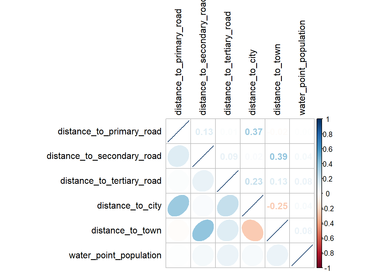
According to Calkins (2005), variables that can be regarded as having a high degree of correlation are indicated by correlation coefficients with magnitudes between ± 0.7 and 1.0. Hence we conclude that there is no highly correlated variables.
Multilogistic Regression
We shall use the glm() function to create our multi logistic regression model, by using status as our explanatory or predictive variable (status) vs the independent variables (our interested data points) using the binomial family and logit link
#status is the variable we are interested as y
model = glm(status ~ distance_to_primary_road + distance_to_secondary_road +
distance_to_tertiary_road + distance_to_city +
distance_to_town + is_urban + usage_capacity +
water_source_clean + water_point_population + local_population_1km,
data = osun_wpt_sf_clean,
family = binomial(link = 'logit')) Instead of using a typical R Report, we use blr_regress() to convert the resulting model into a report
blr_regress(model) Model Overview
------------------------------------------------------------------------
Data Set Resp Var Obs. Df. Model Df. Residual Convergence
------------------------------------------------------------------------
data status 4756 4755 4744 TRUE
------------------------------------------------------------------------
Response Summary
--------------------------------------------------------
Outcome Frequency Outcome Frequency
--------------------------------------------------------
0 2114 1 2642
--------------------------------------------------------
Maximum Likelihood Estimates
-----------------------------------------------------------------------------------------------
Parameter DF Estimate Std. Error z value Pr(>|z|)
-----------------------------------------------------------------------------------------------
(Intercept) 1 -0.2344 0.1240 -1.8903 0.0587
distance_to_primary_road 1 0.0000 0.0000 -0.7153 0.4744
distance_to_secondary_road 1 0.0000 0.0000 -0.5530 0.5802
distance_to_tertiary_road 1 1e-04 0.0000 4.6708 0.0000
distance_to_city 1 0.0000 0.0000 -4.7574 0.0000
distance_to_town 1 0.0000 0.0000 -4.9170 0.0000
is_urbanTRUE 1 -0.2971 0.0819 -3.6294 3e-04
usage_capacitySMALL 1 0.6230 0.0697 8.9366 0.0000
water_source_cleanProtected Shallow Well 1 0.5040 0.0857 5.8783 0.0000
water_source_cleanProtected Spring 1 1.2882 0.4388 2.9359 0.0033
water_point_population 1 -5e-04 0.0000 -11.3686 0.0000
local_population_1km 1 3e-04 0.0000 19.2953 0.0000
-----------------------------------------------------------------------------------------------
Association of Predicted Probabilities and Observed Responses
---------------------------------------------------------------
% Concordant 0.7347 Somers' D 0.4693
% Discordant 0.2653 Gamma 0.4693
% Tied 0.0000 Tau-a 0.2318
Pairs 5585188 c 0.7347
---------------------------------------------------------------We will exclude distance_to_primary_road & distance_to_secondary_road as they have a p value of more than 0.05 implying that they are statistically insignificant
For categorical variable, a positive value implies an above average correlation and a negative value implies a below average correlation
usage_capacity & water_source_clean implies an above average correlation
is_urban implies a below average correlation
For continuous variables, positive value implies a direct correlation and a negative correlation implies an inverse correlation
distance_to_tertiary_road, distance_to_city, distance_to_town, local_population_1km has a direct correlation with the functional status of water points
water_point_population has an inverse correlation with the functional status of water points
We can generate the confusion matrix by using the model with the function blr_confusion_matrix() with a cut off of 0.5 (For fitted values above 0.5, they are functional)
blr_confusion_matrix(model, cutoff = 0.5)Confusion Matrix and Statistics
Reference
Prediction FALSE TRUE
0 1301 738
1 813 1904
Accuracy : 0.6739
No Information Rate : 0.4445
Kappa : 0.3373
McNemars's Test P-Value : 0.0602
Sensitivity : 0.7207
Specificity : 0.6154
Pos Pred Value : 0.7008
Neg Pred Value : 0.6381
Prevalence : 0.5555
Detection Rate : 0.4003
Detection Prevalence : 0.5713
Balanced Accuracy : 0.6680
Precision : 0.7008
Recall : 0.7207
'Positive' Class : 1The accuracy for this Multi logistic regression model is 67.39% has low distinguish ability.
True positive rate (Sensitivity) is at 72.07% while True Negative Rate (Specificity) is quite low at only 61.54%.
This model is not very good to explain or predict functional water points in Osun, we will thus look at Geographically weighted Logistic Regression (GWLR)
Using Geographically Weighted Logistic Regression (GWLR)
First, we must first transform osun_wp_sf_clean into a spatial polygons data frame using as_Spatial(). This is because SP objects (SpatialPointDataFrame) is required to generate the GWLR
osun_wp_sp = osun_wpt_sf_clean %>%
select(var_list) %>%
as_Spatial()Using a fixed distance matrix, we will find the fixed distance bandwidth by using bw.ggwr(), we set longlat to FALSE as the dataframe has already been transformed into the Nigeria Mid Belt projected coordinate system.
bw.fixed = bw.ggwr(status ~ distance_to_primary_road + distance_to_secondary_road +
distance_to_tertiary_road + distance_to_city +
distance_to_town + is_urban + usage_capacity +
water_source_clean + water_point_population + local_population_1km,
data = osun_wp_sp,
family = "binomial",
approach = "AIC",
kernel = "gaussian",
adaptive = FALSE,
longlat = FALSE #use false if its converted into projected coord system (number will be very big)
)Take a cup of tea and have a break, it will take a few minutes.
-----A kind suggestion from GWmodel development group
Iteration Log-Likelihood:(With bandwidth: 95768.67 )
=========================
0 -2889
1 -2836
2 -2830
3 -2829
4 -2829
5 -2829
Fixed bandwidth: 95768.67 AICc value: 5684.357
Iteration Log-Likelihood:(With bandwidth: 59200.13 )
=========================
0 -2875
1 -2818
2 -2810
3 -2808
4 -2808
5 -2808
Fixed bandwidth: 59200.13 AICc value: 5646.785
Iteration Log-Likelihood:(With bandwidth: 36599.53 )
=========================
0 -2847
1 -2781
2 -2768
3 -2765
4 -2765
5 -2765
6 -2765
Fixed bandwidth: 36599.53 AICc value: 5575.148
Iteration Log-Likelihood:(With bandwidth: 22631.59 )
=========================
0 -2798
1 -2719
2 -2698
3 -2693
4 -2693
5 -2693
6 -2693
Fixed bandwidth: 22631.59 AICc value: 5466.883
Iteration Log-Likelihood:(With bandwidth: 13998.93 )
=========================
0 -2720
1 -2622
2 -2590
3 -2581
4 -2580
5 -2580
6 -2580
7 -2580
Fixed bandwidth: 13998.93 AICc value: 5324.578
Iteration Log-Likelihood:(With bandwidth: 8663.649 )
=========================
0 -2601
1 -2476
2 -2431
3 -2419
4 -2417
5 -2417
6 -2417
7 -2417
Fixed bandwidth: 8663.649 AICc value: 5163.61
Iteration Log-Likelihood:(With bandwidth: 5366.266 )
=========================
0 -2436
1 -2268
2 -2194
3 -2167
4 -2161
5 -2161
6 -2161
7 -2161
8 -2161
9 -2161
Fixed bandwidth: 5366.266 AICc value: 4990.587
Iteration Log-Likelihood:(With bandwidth: 3328.371 )
=========================
0 -2157
1 -1922
2 -1802
3 -1739
4 -1713
5 -1713
Fixed bandwidth: 3328.371 AICc value: 4798.288
Iteration Log-Likelihood:(With bandwidth: 2068.882 )
=========================
0 -1751
1 -1421
2 -1238
3 -1133
4 -1084
5 -1084
Fixed bandwidth: 2068.882 AICc value: 4837.017
Iteration Log-Likelihood:(With bandwidth: 4106.777 )
=========================
0 -2297
1 -2095
2 -1997
3 -1951
4 -1938
5 -1936
6 -1936
7 -1936
8 -1936
Fixed bandwidth: 4106.777 AICc value: 4873.161
Iteration Log-Likelihood:(With bandwidth: 2847.289 )
=========================
0 -2036
1 -1771
2 -1633
3 -1558
4 -1525
5 -1525
Fixed bandwidth: 2847.289 AICc value: 4768.192
Iteration Log-Likelihood:(With bandwidth: 2549.964 )
=========================
0 -1941
1 -1655
2 -1503
3 -1417
4 -1378
5 -1378
Fixed bandwidth: 2549.964 AICc value: 4762.212
Iteration Log-Likelihood:(With bandwidth: 2366.207 )
=========================
0 -1874
1 -1573
2 -1410
3 -1316
4 -1274
5 -1274
Fixed bandwidth: 2366.207 AICc value: 4773.081
Iteration Log-Likelihood:(With bandwidth: 2663.532 )
=========================
0 -1979
1 -1702
2 -1555
3 -1474
4 -1438
5 -1438
Fixed bandwidth: 2663.532 AICc value: 4762.568
Iteration Log-Likelihood:(With bandwidth: 2479.775 )
=========================
0 -1917
1 -1625
2 -1468
3 -1380
4 -1339
5 -1339
Fixed bandwidth: 2479.775 AICc value: 4764.294
Iteration Log-Likelihood:(With bandwidth: 2593.343 )
=========================
0 -1956
1 -1674
2 -1523
3 -1439
4 -1401
5 -1401
Fixed bandwidth: 2593.343 AICc value: 4761.813
Iteration Log-Likelihood:(With bandwidth: 2620.153 )
=========================
0 -1965
1 -1685
2 -1536
3 -1453
4 -1415
5 -1415
Fixed bandwidth: 2620.153 AICc value: 4761.89
Iteration Log-Likelihood:(With bandwidth: 2576.774 )
=========================
0 -1950
1 -1667
2 -1515
3 -1431
4 -1393
5 -1393
Fixed bandwidth: 2576.774 AICc value: 4761.889
Iteration Log-Likelihood:(With bandwidth: 2603.584 )
=========================
0 -1960
1 -1678
2 -1528
3 -1445
4 -1407
5 -1407
Fixed bandwidth: 2603.584 AICc value: 4761.813
Iteration Log-Likelihood:(With bandwidth: 2609.913 )
=========================
0 -1962
1 -1680
2 -1531
3 -1448
4 -1410
5 -1410
Fixed bandwidth: 2609.913 AICc value: 4761.831
Iteration Log-Likelihood:(With bandwidth: 2599.672 )
=========================
0 -1958
1 -1676
2 -1526
3 -1443
4 -1405
5 -1405
Fixed bandwidth: 2599.672 AICc value: 4761.809
Iteration Log-Likelihood:(With bandwidth: 2597.255 )
=========================
0 -1957
1 -1675
2 -1525
3 -1441
4 -1403
5 -1403
Fixed bandwidth: 2597.255 AICc value: 4761.809 The fixed bandwidth was found to be 2597.255m or 2.597 km
We will then generate our GWLR model using ggwr.basic()
gwlr.fixed = ggwr.basic(status ~ distance_to_primary_road + distance_to_secondary_road +
distance_to_tertiary_road + distance_to_city +
distance_to_town + is_urban + usage_capacity +
water_source_clean + water_point_population + local_population_1km,
data = osun_wp_sp,
bw = bw.fixed,
family = "binomial",
kernel = "gaussian",
adaptive = FALSE,
longlat = FALSE #use false if its converted into projected coord system (number will be very big)
) Iteration Log-Likelihood
=========================
0 -1958
1 -1676
2 -1526
3 -1443
4 -1405
5 -1405 Lets check the result by displaying gwlr.fixed
gwlr.fixed ***********************************************************************
* Package GWmodel *
***********************************************************************
Program starts at: 2023-01-04 19:48:19
Call:
ggwr.basic(formula = status ~ distance_to_primary_road + distance_to_secondary_road +
distance_to_tertiary_road + distance_to_city + distance_to_town +
is_urban + usage_capacity + water_source_clean + water_point_population +
local_population_1km, data = osun_wp_sp, bw = bw.fixed, family = "binomial",
kernel = "gaussian", adaptive = FALSE, longlat = FALSE)
Dependent (y) variable: status
Independent variables: distance_to_primary_road distance_to_secondary_road distance_to_tertiary_road distance_to_city distance_to_town is_urban usage_capacity water_source_clean water_point_population local_population_1km
Number of data points: 4756
Used family: binomial
***********************************************************************
* Results of Generalized linear Regression *
***********************************************************************
Call:
NULL
Deviance Residuals:
Min 1Q Median 3Q Max
-124.555 -1.755 1.072 1.742 34.333
Coefficients:
Estimate Std. Error z value Pr(>|z|)
Intercept -2.344e-01 1.240e-01 -1.890 0.058713
distance_to_primary_road -4.642e-06 6.490e-06 -0.715 0.474422
distance_to_secondary_road -5.143e-06 9.299e-06 -0.553 0.580230
distance_to_tertiary_road 9.683e-05 2.073e-05 4.671 3.00e-06
distance_to_city -1.686e-05 3.544e-06 -4.757 1.96e-06
distance_to_town -1.480e-05 3.009e-06 -4.917 8.79e-07
is_urbanTRUE -2.971e-01 8.185e-02 -3.629 0.000284
usage_capacitySMALL 6.230e-01 6.972e-02 8.937 < 2e-16
water_source_cleanProtected Shallow Well 5.040e-01 8.574e-02 5.878 4.14e-09
water_source_cleanProtected Spring 1.288e+00 4.388e-01 2.936 0.003325
water_point_population -5.097e-04 4.484e-05 -11.369 < 2e-16
local_population_1km 3.451e-04 1.788e-05 19.295 < 2e-16
Intercept .
distance_to_primary_road
distance_to_secondary_road
distance_to_tertiary_road ***
distance_to_city ***
distance_to_town ***
is_urbanTRUE ***
usage_capacitySMALL ***
water_source_cleanProtected Shallow Well ***
water_source_cleanProtected Spring **
water_point_population ***
local_population_1km ***
---
Signif. codes: 0 '***' 0.001 '**' 0.01 '*' 0.05 '.' 0.1 ' ' 1
(Dispersion parameter for binomial family taken to be 1)
Null deviance: 6534.5 on 4755 degrees of freedom
Residual deviance: 5688.0 on 4744 degrees of freedom
AIC: 5712
Number of Fisher Scoring iterations: 5
AICc: 5712.099
Pseudo R-square value: 0.1295351
***********************************************************************
* Results of Geographically Weighted Regression *
***********************************************************************
*********************Model calibration information*********************
Kernel function: gaussian
Fixed bandwidth: 2599.672
Regression points: the same locations as observations are used.
Distance metric: A distance matrix is specified for this model calibration.
************Summary of Generalized GWR coefficient estimates:**********
Min. 1st Qu. Median
Intercept -8.7269e+02 -5.4465e+00 1.1507e+00
distance_to_primary_road -1.9389e-02 -4.8031e-04 2.9618e-05
distance_to_secondary_road -1.5921e-02 -3.7551e-04 1.2317e-04
distance_to_tertiary_road -1.5618e-02 -4.2368e-04 7.6179e-05
distance_to_city -1.8416e-02 -5.6217e-04 -1.2726e-04
distance_to_town -2.2411e-02 -5.7283e-04 -1.5155e-04
is_urbanTRUE -1.9790e+02 -4.2908e+00 -1.6864e+00
usage_capacitySMALL -5.9281e+00 -3.0322e-01 4.1592e-01
water_source_cleanProtected.Shallow.Well -2.0789e+01 -4.5190e-01 5.3340e-01
water_source_cleanProtected.Spring -5.2235e+02 -5.5977e+00 2.5441e+00
water_point_population -5.2208e-02 -2.2767e-03 -9.8875e-04
local_population_1km -1.2698e-01 4.9952e-04 1.0638e-03
3rd Qu. Max.
Intercept 1.2248e+01 1063.6697
distance_to_primary_road 4.8443e-04 0.0142
distance_to_secondary_road 6.0692e-04 0.0258
distance_to_tertiary_road 6.6814e-04 0.0128
distance_to_city 2.3718e-04 0.0150
distance_to_town 1.9271e-04 0.0224
is_urbanTRUE 1.2841e+00 744.3097
usage_capacitySMALL 9.7231e-01 20.7720
water_source_cleanProtected.Shallow.Well 1.7849e+00 67.6343
water_source_cleanProtected.Spring 6.7663e+00 317.4123
water_point_population 5.0102e-04 0.1309
local_population_1km 1.8157e-03 0.0392
************************Diagnostic information*************************
Number of data points: 4756
GW Deviance: 2795.084
AIC : 4414.606
AICc : 4747.423
Pseudo R-square value: 0.5722559
***********************************************************************
Program stops at: 2023-01-04 19:48:52 The AIC value of Geographically Weighted Logistic Regression (GWLR) is 4414.606 vs Generalized Linear regression model (GLR) at 5712. Hence, we can conclude that there is a significant improvement on the GWLR model, with a difference of about 1297.
To assess the performance of GWLR , we need to first convert the SDF object as a data frame
gwr.fixed = as.data.frame(gwlr.fixed$SDF)Next, we will label yhat values greater or equal to 0.5 into 1 and 0 otherwise into the most column by using mutate() to denote functional water points.
gwr.fixed = gwr.fixed %>%
mutate(most =
ifelse(gwr.fixed$yhat >= 0.5, T, F))We then generate the confusion matrix for both functional and non functional water points.
gwr.fixed$y = as.factor(gwr.fixed$y)
gwr.fixed$most = as.factor(gwr.fixed$most)
cm_func = confusionMatrix(data = gwr.fixed$most,
reference = gwr.fixed$y)
cm_funcConfusion Matrix and Statistics
Reference
Prediction FALSE TRUE
FALSE 1824 263
TRUE 290 2379
Accuracy : 0.8837
95% CI : (0.8743, 0.8927)
No Information Rate : 0.5555
P-Value [Acc > NIR] : <2e-16
Kappa : 0.7642
Mcnemar's Test P-Value : 0.2689
Sensitivity : 0.8628
Specificity : 0.9005
Pos Pred Value : 0.8740
Neg Pred Value : 0.8913
Prevalence : 0.4445
Detection Rate : 0.3835
Detection Prevalence : 0.4388
Balanced Accuracy : 0.8816
'Positive' Class : FALSE
Comparing the Confusion matrix with the Multilogistic Regression model, the accuracy has significantly increase from 67.39% to 88.37%, sensitivity (True positive rate) increased from 72.07% to 86.28% and specificity (True negative rate) increased from 61.54% to 90.05%, for the GWLR model.
Visualizing the results of GWLR
We select our variable of interested by using the select() function, and then bind the data frame with osun_wpt_sf_selected with the GWLR data frame gwr.fixed
Thereafter, we create a multi layer map with tmap by using the Osun Map as base, followed by the yhat variable to plot the water points, with fixed breaks of 0, 0.5 and 1.0.
Lastly, we plot the LGA of OSun to figure out which LGAs requires attention
osun_wpt_sf_selected = osun_wpt_sf_clean %>%
select(c(ADM2_EN, ADM2_PCODE, ADM1_EN, ADM1_PCODE, status))
gwr_sf.fixed = cbind(osun_wpt_sf_selected, gwr.fixed)
prob_t = tm_shape(osun) +
tm_polygons(alpha = 0.1) +
tm_shape(gwr_sf.fixed) +
tm_dots(col="yhat", n = 3, breaks = c(0, 0.50, 1.00),
style = "fixed",
border.col = "gray60",
border.lwd = 1) +
tm_shape(osun) +
tm_polygons(col="ADM2_EN", alpha = 0.2) +
tm_view(set.zoom.limits = c(9,14))
prob_tIn this model, we can observe that the area of concern in Osun as shown by the plot above. It can be observed that the North West region of Osun has a high concentration of non functional water points as compared to the rest of the LGAs. Significant areas includes Ejigbo, Egbedore, Ede North, Ede South and Ola-oluwa.
Optimizing our GWLR model
Since we now know that the 2 variables distance_to_primary_road and distance_to_secondary_road is statistically insignificant, we shall optimize the model by removing the 2 variables in our GWLR model.
Similarly, in the previous section, we will use a fixed distance matrix, we will find the fixed distance bandwidth by using bw.ggwr(), we set longlat to FALSE as the data frame has already been transformed into the Nigeria Mid Belt projected coordinate system.
bw.sigvar.fixed = bw.ggwr(status ~ distance_to_tertiary_road + distance_to_city +
distance_to_town + is_urban + usage_capacity +
water_source_clean + water_point_population + local_population_1km,
data = osun_wp_sp,
family = "binomial",
approach = "AIC",
kernel = "gaussian",
adaptive = FALSE,
longlat = FALSE #use false if its converted into projected coord system (number will be very big)
)Take a cup of tea and have a break, it will take a few minutes.
-----A kind suggestion from GWmodel development group
Iteration Log-Likelihood:(With bandwidth: 95768.67 )
=========================
0 -2890
1 -2837
2 -2830
3 -2829
4 -2829
5 -2829
Fixed bandwidth: 95768.67 AICc value: 5681.18
Iteration Log-Likelihood:(With bandwidth: 59200.13 )
=========================
0 -2878
1 -2820
2 -2812
3 -2810
4 -2810
5 -2810
Fixed bandwidth: 59200.13 AICc value: 5645.901
Iteration Log-Likelihood:(With bandwidth: 36599.53 )
=========================
0 -2854
1 -2790
2 -2777
3 -2774
4 -2774
5 -2774
6 -2774
Fixed bandwidth: 36599.53 AICc value: 5585.354
Iteration Log-Likelihood:(With bandwidth: 22631.59 )
=========================
0 -2810
1 -2732
2 -2711
3 -2707
4 -2707
5 -2707
6 -2707
Fixed bandwidth: 22631.59 AICc value: 5481.877
Iteration Log-Likelihood:(With bandwidth: 13998.93 )
=========================
0 -2732
1 -2635
2 -2604
3 -2597
4 -2596
5 -2596
6 -2596
Fixed bandwidth: 13998.93 AICc value: 5333.718
Iteration Log-Likelihood:(With bandwidth: 8663.649 )
=========================
0 -2624
1 -2502
2 -2459
3 -2447
4 -2446
5 -2446
6 -2446
7 -2446
Fixed bandwidth: 8663.649 AICc value: 5178.493
Iteration Log-Likelihood:(With bandwidth: 5366.266 )
=========================
0 -2478
1 -2319
2 -2250
3 -2225
4 -2219
5 -2219
6 -2220
7 -2220
8 -2220
9 -2220
Fixed bandwidth: 5366.266 AICc value: 5022.016
Iteration Log-Likelihood:(With bandwidth: 3328.371 )
=========================
0 -2222
1 -2002
2 -1894
3 -1838
4 -1818
5 -1814
6 -1814
Fixed bandwidth: 3328.371 AICc value: 4827.587
Iteration Log-Likelihood:(With bandwidth: 2068.882 )
=========================
0 -1837
1 -1528
2 -1357
3 -1261
4 -1222
5 -1222
Fixed bandwidth: 2068.882 AICc value: 4772.046
Iteration Log-Likelihood:(With bandwidth: 1290.476 )
=========================
0 -1403
1 -1016
2 -807.3
3 -680.2
4 -680.2
Fixed bandwidth: 1290.476 AICc value: 5808.015
Iteration Log-Likelihood:(With bandwidth: 2549.964 )
=========================
0 -2019
1 -1753
2 -1614
3 -1538
4 -1506
5 -1506
Fixed bandwidth: 2549.964 AICc value: 4764.056
Iteration Log-Likelihood:(With bandwidth: 2847.289 )
=========================
0 -2108
1 -1862
2 -1736
3 -1670
4 -1644
5 -1644
Fixed bandwidth: 2847.289 AICc value: 4791.834
Iteration Log-Likelihood:(With bandwidth: 2366.207 )
=========================
0 -1955
1 -1675
2 -1525
3 -1441
4 -1407
5 -1407
Fixed bandwidth: 2366.207 AICc value: 4755.524
Iteration Log-Likelihood:(With bandwidth: 2252.639 )
=========================
0 -1913
1 -1623
2 -1465
3 -1376
4 -1341
5 -1341
Fixed bandwidth: 2252.639 AICc value: 4759.188
Iteration Log-Likelihood:(With bandwidth: 2436.396 )
=========================
0 -1980
1 -1706
2 -1560
3 -1479
4 -1446
5 -1446
Fixed bandwidth: 2436.396 AICc value: 4756.675
Iteration Log-Likelihood:(With bandwidth: 2322.828 )
=========================
0 -1940
1 -1656
2 -1503
3 -1417
4 -1382
5 -1382
Fixed bandwidth: 2322.828 AICc value: 4756.471
Iteration Log-Likelihood:(With bandwidth: 2393.017 )
=========================
0 -1965
1 -1687
2 -1539
3 -1456
4 -1422
5 -1422
Fixed bandwidth: 2393.017 AICc value: 4755.57
Iteration Log-Likelihood:(With bandwidth: 2349.638 )
=========================
0 -1949
1 -1668
2 -1517
3 -1432
4 -1398
5 -1398
Fixed bandwidth: 2349.638 AICc value: 4755.753
Iteration Log-Likelihood:(With bandwidth: 2376.448 )
=========================
0 -1959
1 -1680
2 -1530
3 -1447
4 -1413
5 -1413
Fixed bandwidth: 2376.448 AICc value: 4755.48
Iteration Log-Likelihood:(With bandwidth: 2382.777 )
=========================
0 -1961
1 -1683
2 -1534
3 -1450
4 -1416
5 -1416
Fixed bandwidth: 2382.777 AICc value: 4755.491
Iteration Log-Likelihood:(With bandwidth: 2372.536 )
=========================
0 -1958
1 -1678
2 -1528
3 -1445
4 -1411
5 -1411
Fixed bandwidth: 2372.536 AICc value: 4755.488
Iteration Log-Likelihood:(With bandwidth: 2378.865 )
=========================
0 -1960
1 -1681
2 -1532
3 -1448
4 -1414
5 -1414
Fixed bandwidth: 2378.865 AICc value: 4755.481
Iteration Log-Likelihood:(With bandwidth: 2374.954 )
=========================
0 -1959
1 -1679
2 -1530
3 -1446
4 -1412
5 -1412
Fixed bandwidth: 2374.954 AICc value: 4755.482
Iteration Log-Likelihood:(With bandwidth: 2377.371 )
=========================
0 -1959
1 -1680
2 -1531
3 -1447
4 -1413
5 -1413
Fixed bandwidth: 2377.371 AICc value: 4755.48
Iteration Log-Likelihood:(With bandwidth: 2377.942 )
=========================
0 -1960
1 -1680
2 -1531
3 -1448
4 -1414
5 -1414
Fixed bandwidth: 2377.942 AICc value: 4755.48
Iteration Log-Likelihood:(With bandwidth: 2377.018 )
=========================
0 -1959
1 -1680
2 -1531
3 -1447
4 -1413
5 -1413
Fixed bandwidth: 2377.018 AICc value: 4755.48 The fixed bandwidth was found to be 2377.018 m or 2.377 km
We will then generate our GWLR model using ggwr.basic()
gwlr.sigvar.fixed = ggwr.basic(status ~ distance_to_tertiary_road + distance_to_city +
distance_to_town + is_urban + usage_capacity +
water_source_clean + water_point_population + local_population_1km,
data = osun_wp_sp,
bw = bw.sigvar.fixed,
family = "binomial",
kernel = "gaussian",
adaptive = FALSE,
longlat = FALSE
) Iteration Log-Likelihood
=========================
0 -1959
1 -1680
2 -1531
3 -1447
4 -1413
5 -1413 Lets check the result by displaying gwlr.sigvar.fixed
gwlr.sigvar.fixed ***********************************************************************
* Package GWmodel *
***********************************************************************
Program starts at: 2023-01-04 19:58:34
Call:
ggwr.basic(formula = status ~ distance_to_tertiary_road + distance_to_city +
distance_to_town + is_urban + usage_capacity + water_source_clean +
water_point_population + local_population_1km, data = osun_wp_sp,
bw = bw.sigvar.fixed, family = "binomial", kernel = "gaussian",
adaptive = FALSE, longlat = FALSE)
Dependent (y) variable: status
Independent variables: distance_to_tertiary_road distance_to_city distance_to_town is_urban usage_capacity water_source_clean water_point_population local_population_1km
Number of data points: 4756
Used family: binomial
***********************************************************************
* Results of Generalized linear Regression *
***********************************************************************
Call:
NULL
Deviance Residuals:
Min 1Q Median 3Q Max
-129.368 -1.750 1.074 1.742 34.126
Coefficients:
Estimate Std. Error z value Pr(>|z|)
Intercept -2.666e-01 1.187e-01 -2.246 0.024716
distance_to_tertiary_road 1.001e-04 2.040e-05 4.910 9.13e-07
distance_to_city -1.764e-05 3.391e-06 -5.202 1.97e-07
distance_to_town -1.544e-05 2.825e-06 -5.466 4.60e-08
is_urbanTRUE -2.667e-01 7.474e-02 -3.569 0.000358
usage_capacitySMALL 6.206e-01 6.966e-02 8.908 < 2e-16
water_source_cleanProtected Shallow Well 4.947e-01 8.496e-02 5.823 5.79e-09
water_source_cleanProtected Spring 1.279e+00 4.384e-01 2.917 0.003530
water_point_population -5.098e-04 4.476e-05 -11.390 < 2e-16
local_population_1km 3.452e-04 1.779e-05 19.407 < 2e-16
Intercept *
distance_to_tertiary_road ***
distance_to_city ***
distance_to_town ***
is_urbanTRUE ***
usage_capacitySMALL ***
water_source_cleanProtected Shallow Well ***
water_source_cleanProtected Spring **
water_point_population ***
local_population_1km ***
---
Signif. codes: 0 '***' 0.001 '**' 0.01 '*' 0.05 '.' 0.1 ' ' 1
(Dispersion parameter for binomial family taken to be 1)
Null deviance: 6534.5 on 4755 degrees of freedom
Residual deviance: 5688.9 on 4746 degrees of freedom
AIC: 5708.9
Number of Fisher Scoring iterations: 5
AICc: 5708.923
Pseudo R-square value: 0.129406
***********************************************************************
* Results of Geographically Weighted Regression *
***********************************************************************
*********************Model calibration information*********************
Kernel function: gaussian
Fixed bandwidth: 2377.371
Regression points: the same locations as observations are used.
Distance metric: A distance matrix is specified for this model calibration.
************Summary of Generalized GWR coefficient estimates:**********
Min. 1st Qu. Median
Intercept -3.6547e+02 -5.0121e+00 3.1882e+00
distance_to_tertiary_road -3.1622e-02 -4.5462e-04 9.1291e-05
distance_to_city -5.4555e-02 -6.5623e-04 -1.3507e-04
distance_to_town -8.6549e-03 -5.2754e-04 -1.6785e-04
is_urbanTRUE -7.3554e+02 -3.4675e+00 -1.6596e+00
usage_capacitySMALL -9.2449e+00 -3.9113e-01 4.1960e-01
water_source_cleanProtected.Shallow.Well -1.8842e+02 -4.7295e-01 6.2378e-01
water_source_cleanProtected.Spring -1.3630e+03 -5.3436e+00 2.7714e+00
water_point_population -2.9696e-02 -2.2705e-03 -1.2277e-03
local_population_1km -7.7730e-02 4.4281e-04 1.0548e-03
3rd Qu. Max.
Intercept 1.3662e+01 2170.9863
distance_to_tertiary_road 6.3011e-04 0.0237
distance_to_city 1.5921e-04 0.0162
distance_to_town 2.4490e-04 0.0179
is_urbanTRUE 1.0554e+00 995.1840
usage_capacitySMALL 1.0347e+00 55.8887
water_source_cleanProtected.Shallow.Well 1.9564e+00 66.8914
water_source_cleanProtected.Spring 7.0805e+00 208.3749
water_point_population 4.5879e-04 0.0765
local_population_1km 1.8479e-03 0.0333
************************Diagnostic information*************************
Number of data points: 4756
GW Deviance: 2815.659
AIC : 4418.776
AICc : 4744.213
Pseudo R-square value: 0.5691072
***********************************************************************
Program stops at: 2023-01-04 19:59:02 The AIC value of Geographically Weighted Logistic Regression (GWLR) is 4418.776 vs Generalized Linear regression model (GLR) at 5708.9. Hence, we can conclude that there is a significant improvement on the GWLR model, with a difference of about 1290.
We can observe that after the 2 statistically insignificant variables were removed, it did not really change the statistical power as the difference between the AIC of the optimized and un-optimized model only differ by 7.
Note: In general, when an independent variable was removed from a regression model, the overall explanatory or performance of the model will be compromised.
This is the nature of regression models. However, when an insignificant independent variable was removed from the model, we should expect the impact on the performance of the model will be lesser than when a significant independent was removed from the model.
To assess the performance of the optimized GWLR, we need to first convert the SDF object as a data frame
gwlr.sigvar.fixed = as.data.frame(gwlr.sigvar.fixed$SDF)Next, we will label yhat values greater or equal to 0.5 into 1 and 0 otherwise into the most column by using mutate() to denote functional water points.
gwlr.sigvar.fixed = gwlr.sigvar.fixed %>%
mutate(most =
ifelse(gwlr.sigvar.fixed$yhat >= 0.5, T, F))We then generate the confusion matrix for both functional and non functional water points.
gwlr.sigvar.fixed$y = as.factor(gwlr.sigvar.fixed$y)
gwlr.sigvar.fixed$most = as.factor(gwlr.sigvar.fixed$most)
cm_func_sigvar = confusionMatrix(data = gwlr.sigvar.fixed$most,
reference = gwlr.sigvar.fixed$y)
cm_func_sigvarConfusion Matrix and Statistics
Reference
Prediction FALSE TRUE
FALSE 1833 268
TRUE 281 2374
Accuracy : 0.8846
95% CI : (0.8751, 0.8935)
No Information Rate : 0.5555
P-Value [Acc > NIR] : <2e-16
Kappa : 0.7661
Mcnemar's Test P-Value : 0.6085
Sensitivity : 0.8671
Specificity : 0.8986
Pos Pred Value : 0.8724
Neg Pred Value : 0.8942
Prevalence : 0.4445
Detection Rate : 0.3854
Detection Prevalence : 0.4418
Balanced Accuracy : 0.8828
'Positive' Class : FALSE
Comparing the Confusion matrix with the Multilogistic Regression model, the accuracy has significantly increase from 67.39% to 88.46%, sensitivity (True positive rate) increased from 72.07% to 86.71% and specificity (True negative rate) increased from 61.54% to 89.86%, for the optimized GWLR model.
Comparing the Confusion matrix with the un-optimized GWLR model, the accuracy has only increased slightly from 88.37% to 88.46% (0.09%), sensitivity (True positive rate) increased slightly from 86.28% to 86.71% (0.43%) and specificity (True negative rate) decreased from 90.05% to 89.86% (0.19%).
This tells us that statistically insignificant variables will not affect the overall performance of GWLR.
Visualizing the results of the optimized GWLR
Similarly, in this case, we select our variable of interested by using the select() function, and then bind the data frame with osun_wpt_sf_selected with the GWLR data frame gwr_sf_sigvar.fixed
Thereafter, we create a multi layer map with tmap by using the Osun Map as base, followed by the yhat variable to plot the water points, with fixed breaks of 0, 0.5 and 1.0.
Lastly, we plot the LGA of OSun to figure out which LGAs requires attention
gwr_sf_sigvar.fixed = cbind(osun_wpt_sf_selected, gwlr.sigvar.fixed)
prob_t_sigvar = tm_shape(osun) +
tm_polygons(alpha = 0.1) +
tm_shape(gwr_sf_sigvar.fixed) +
tm_dots(col="yhat", n = 3, breaks = c(0, 0.50, 1.00),
style = "fixed",
border.col = "gray60",
border.lwd = 1) +
tm_shape(osun) +
tm_polygons(col="ADM2_EN", alpha = 0.2) +
tm_view(set.zoom.limits = c(9,14))
prob_t_sigvarWe will plot both the optimized and un-optimized GWLR models side by side using tmap_arrange() to determine if there is any significant difference visually
tmap_arrange(prob_t, prob_t_sigvar,
ncol = 2, nrow = 1, asp = 1,
sync = TRUE)From the above the plot, both the models presents similar trends that the north west region of Osun deserves attention as it presents a high concentration of non functional water points as compared to the rest of the LGAs.
Conclusion
The Nigerian government should use a localized strategy at the state level rather than a national strategy to address the issue of water points functionality, based on the considerable increase from both the optimized and un-optimized GWLR model. To increase access to water in Nigeria’s rural areas, state governments will have to take analyze data at the state level while receiving overarching federal guidance.
References
Calkins K. G (2005) Applied Statistics - Lesson 5, Correlation Coefficients
https://www.andrews.edu/~calkins/math/edrm611/edrm05.htm#:~:text=Correlation%20coefficients%20whose%20magnitude%20are,can%20be%20considered%20highly%20correlated.