pacman::p_load(olsrr, corrplot, ggpubr, sf, spdep, GWmodel, tmap, tidyverse, gtsummary)In class exercise 4 - Hedonic Pricing Models using GWR and Visualizing coefficient estimates of 2015 Condo Resale price in Singapore
Overview
Geographically weighted regression (GWR) is a spatial statistical technique that models the local relationships between these independent variables and an outcome of interest while taking non-stationary variables (such as climate, demographic factors, and physical environment characteristics) into account (also known as dependent variable).
We will practice using GWR techniques to construct Hedonic pricing models in this practical exercise.
The 2015 condominium resale prices is the dependent variable. There are two categories of independent variables: structural and locational.
Two data sets will be used in this model building exercise, they are:
URA Master Plan subzone boundary in shapefile format (i.e. MP14_SUBZONE_WEB_PL)
condo_resale_2015 in csv format (i.e. condo_resale_2015.csv)
Getting Started
Before we begin, we need to install the necessary R packages into R and launch them in the R environment
The R packages requirements for this exercise are:
R package for building OLS and performing diagnostics tests
R package for calibrating geographical weighted family of models
R package for multivariate data visualisation and analysis
Spatial data handling
- sf
Attribute data handling
- tidyverse, especially readr, ggplot2 and dplyr
Choropleth mapping
- tmap
We load the required packages in R with the code below.
What is in the GWModel Package
The GWmodel package offers a variety of localized spatial statistical methods, including GW summary statistics, GW principle components analysis, GW discriminant analysis, and other types of GW regression, some of which are offered in simple and reliable (outlier resistant) forms.
A handy exploratory tool that frequently comes before (and directs) a more conventional or complex statistical analysis is provided by mapping the outputs or parameters of the GWmodel.
Spatial Data
Loading the Master Plan 2014 Subzone Boundary
We will load the spatial data using st_read()
mpsz = st_read(dsn="data/geospatial", layer="MP14_SUBZONE_WEB_PL")Reading layer `MP14_SUBZONE_WEB_PL' from data source
`D:\Allanckw\ISSS624\In-Class_Ex4\data\geospatial' using driver `ESRI Shapefile'
Simple feature collection with 323 features and 15 fields
Geometry type: MULTIPOLYGON
Dimension: XY
Bounding box: xmin: 2667.538 ymin: 15748.72 xmax: 56396.44 ymax: 50256.33
Projected CRS: SVY21By using st_crs() to inspect the sf object, the dataframe is still in WGS84 format. As such we will need to transform it to the SVY21 projection system by calling st_transform()
st_crs(mpsz)Coordinate Reference System:
User input: SVY21
wkt:
PROJCRS["SVY21",
BASEGEOGCRS["SVY21[WGS84]",
DATUM["World Geodetic System 1984",
ELLIPSOID["WGS 84",6378137,298.257223563,
LENGTHUNIT["metre",1]],
ID["EPSG",6326]],
PRIMEM["Greenwich",0,
ANGLEUNIT["Degree",0.0174532925199433]]],
CONVERSION["unnamed",
METHOD["Transverse Mercator",
ID["EPSG",9807]],
PARAMETER["Latitude of natural origin",1.36666666666667,
ANGLEUNIT["Degree",0.0174532925199433],
ID["EPSG",8801]],
PARAMETER["Longitude of natural origin",103.833333333333,
ANGLEUNIT["Degree",0.0174532925199433],
ID["EPSG",8802]],
PARAMETER["Scale factor at natural origin",1,
SCALEUNIT["unity",1],
ID["EPSG",8805]],
PARAMETER["False easting",28001.642,
LENGTHUNIT["metre",1],
ID["EPSG",8806]],
PARAMETER["False northing",38744.572,
LENGTHUNIT["metre",1],
ID["EPSG",8807]]],
CS[Cartesian,2],
AXIS["(E)",east,
ORDER[1],
LENGTHUNIT["metre",1,
ID["EPSG",9001]]],
AXIS["(N)",north,
ORDER[2],
LENGTHUNIT["metre",1,
ID["EPSG",9001]]]]mpsz_svy21 = st_transform(mpsz, 3414)
st_crs(mpsz_svy21)Coordinate Reference System:
User input: EPSG:3414
wkt:
PROJCRS["SVY21 / Singapore TM",
BASEGEOGCRS["SVY21",
DATUM["SVY21",
ELLIPSOID["WGS 84",6378137,298.257223563,
LENGTHUNIT["metre",1]]],
PRIMEM["Greenwich",0,
ANGLEUNIT["degree",0.0174532925199433]],
ID["EPSG",4757]],
CONVERSION["Singapore Transverse Mercator",
METHOD["Transverse Mercator",
ID["EPSG",9807]],
PARAMETER["Latitude of natural origin",1.36666666666667,
ANGLEUNIT["degree",0.0174532925199433],
ID["EPSG",8801]],
PARAMETER["Longitude of natural origin",103.833333333333,
ANGLEUNIT["degree",0.0174532925199433],
ID["EPSG",8802]],
PARAMETER["Scale factor at natural origin",1,
SCALEUNIT["unity",1],
ID["EPSG",8805]],
PARAMETER["False easting",28001.642,
LENGTHUNIT["metre",1],
ID["EPSG",8806]],
PARAMETER["False northing",38744.572,
LENGTHUNIT["metre",1],
ID["EPSG",8807]]],
CS[Cartesian,2],
AXIS["northing (N)",north,
ORDER[1],
LENGTHUNIT["metre",1]],
AXIS["easting (E)",east,
ORDER[2],
LENGTHUNIT["metre",1]],
USAGE[
SCOPE["Cadastre, engineering survey, topographic mapping."],
AREA["Singapore - onshore and offshore."],
BBOX[1.13,103.59,1.47,104.07]],
ID["EPSG",3414]]From inspection, we know that mpsz_svy21 is now referencing the correct projection system.
Aspatial Data
To load the raw condo_resale_2015.csv data file, we use the read_csv function to import condo_resale_2015 into R as a tibble data frame named condo_resale.
condo_resale = read_csv("data/aspatial/Condo_resale_2015.csv")It’s necessary that we check to see if the data file was successfully imported into R after importing it. We can use the glimpse() function to achieve that
glimpse(condo_resale)Rows: 1,436
Columns: 23
$ LATITUDE <dbl> 1.287145, 1.328698, 1.313727, 1.308563, 1.321437,…
$ LONGITUDE <dbl> 103.7802, 103.8123, 103.7971, 103.8247, 103.9505,…
$ POSTCODE <dbl> 118635, 288420, 267833, 258380, 467169, 466472, 3…
$ SELLING_PRICE <dbl> 3000000, 3880000, 3325000, 4250000, 1400000, 1320…
$ AREA_SQM <dbl> 309, 290, 248, 127, 145, 139, 218, 141, 165, 168,…
$ AGE <dbl> 30, 32, 33, 7, 28, 22, 24, 24, 27, 31, 17, 22, 6,…
$ PROX_CBD <dbl> 7.941259, 6.609797, 6.898000, 4.038861, 11.783402…
$ PROX_CHILDCARE <dbl> 0.16597932, 0.28027246, 0.42922669, 0.39473543, 0…
$ PROX_ELDERLYCARE <dbl> 2.5198118, 1.9333338, 0.5021395, 1.9910316, 1.121…
$ PROX_URA_GROWTH_AREA <dbl> 6.618741, 7.505109, 6.463887, 4.906512, 6.410632,…
$ PROX_HAWKER_MARKET <dbl> 1.76542207, 0.54507614, 0.37789301, 1.68259969, 0…
$ PROX_KINDERGARTEN <dbl> 0.05835552, 0.61592412, 0.14120309, 0.38200076, 0…
$ PROX_MRT <dbl> 0.5607188, 0.6584461, 0.3053433, 0.6910183, 0.528…
$ PROX_PARK <dbl> 1.1710446, 0.1992269, 0.2779886, 0.9832843, 0.116…
$ PROX_PRIMARY_SCH <dbl> 1.6340256, 0.9747834, 1.4715016, 1.4546324, 0.709…
$ PROX_TOP_PRIMARY_SCH <dbl> 3.3273195, 0.9747834, 1.4715016, 2.3006394, 0.709…
$ PROX_SHOPPING_MALL <dbl> 2.2102717, 2.9374279, 1.2256850, 0.3525671, 1.307…
$ PROX_SUPERMARKET <dbl> 0.9103958, 0.5900617, 0.4135583, 0.4162219, 0.581…
$ PROX_BUS_STOP <dbl> 0.10336166, 0.28673408, 0.28504777, 0.29872340, 0…
$ NO_Of_UNITS <dbl> 18, 20, 27, 30, 30, 31, 32, 32, 32, 32, 34, 34, 3…
$ FAMILY_FRIENDLY <dbl> 0, 0, 0, 0, 0, 1, 1, 0, 1, 1, 0, 0, 0, 0, 0, 0, 0…
$ FREEHOLD <dbl> 1, 1, 1, 1, 1, 1, 1, 1, 1, 0, 1, 1, 1, 1, 1, 1, 1…
$ LEASEHOLD_99YR <dbl> 0, 0, 0, 0, 0, 0, 0, 0, 0, 0, 0, 0, 0, 0, 0, 0, 0…Creating a feature dataframe from an Aspatial data frame with st_as_sf()
We can use st_as_sfto create a data frame from the LONGITUDE (x) and LATITUDE (y) values. The EPSG 4326 code is used as the dataset is referencing WGS84 geographic coordinate system.
We will need to call st_transform() such that it will be the same projection system as the mpsz_svy21 spatial feature data frame
condo_resale_sf = st_as_sf(condo_resale, coords = c("LONGITUDE", "LATITUDE"),
crs=4326) %>%
st_transform(crs=3414)
glimpse(condo_resale_sf)Rows: 1,436
Columns: 22
$ POSTCODE <dbl> 118635, 288420, 267833, 258380, 467169, 466472, 3…
$ SELLING_PRICE <dbl> 3000000, 3880000, 3325000, 4250000, 1400000, 1320…
$ AREA_SQM <dbl> 309, 290, 248, 127, 145, 139, 218, 141, 165, 168,…
$ AGE <dbl> 30, 32, 33, 7, 28, 22, 24, 24, 27, 31, 17, 22, 6,…
$ PROX_CBD <dbl> 7.941259, 6.609797, 6.898000, 4.038861, 11.783402…
$ PROX_CHILDCARE <dbl> 0.16597932, 0.28027246, 0.42922669, 0.39473543, 0…
$ PROX_ELDERLYCARE <dbl> 2.5198118, 1.9333338, 0.5021395, 1.9910316, 1.121…
$ PROX_URA_GROWTH_AREA <dbl> 6.618741, 7.505109, 6.463887, 4.906512, 6.410632,…
$ PROX_HAWKER_MARKET <dbl> 1.76542207, 0.54507614, 0.37789301, 1.68259969, 0…
$ PROX_KINDERGARTEN <dbl> 0.05835552, 0.61592412, 0.14120309, 0.38200076, 0…
$ PROX_MRT <dbl> 0.5607188, 0.6584461, 0.3053433, 0.6910183, 0.528…
$ PROX_PARK <dbl> 1.1710446, 0.1992269, 0.2779886, 0.9832843, 0.116…
$ PROX_PRIMARY_SCH <dbl> 1.6340256, 0.9747834, 1.4715016, 1.4546324, 0.709…
$ PROX_TOP_PRIMARY_SCH <dbl> 3.3273195, 0.9747834, 1.4715016, 2.3006394, 0.709…
$ PROX_SHOPPING_MALL <dbl> 2.2102717, 2.9374279, 1.2256850, 0.3525671, 1.307…
$ PROX_SUPERMARKET <dbl> 0.9103958, 0.5900617, 0.4135583, 0.4162219, 0.581…
$ PROX_BUS_STOP <dbl> 0.10336166, 0.28673408, 0.28504777, 0.29872340, 0…
$ NO_Of_UNITS <dbl> 18, 20, 27, 30, 30, 31, 32, 32, 32, 32, 34, 34, 3…
$ FAMILY_FRIENDLY <dbl> 0, 0, 0, 0, 0, 1, 1, 0, 1, 1, 0, 0, 0, 0, 0, 0, 0…
$ FREEHOLD <dbl> 1, 1, 1, 1, 1, 1, 1, 1, 1, 0, 1, 1, 1, 1, 1, 1, 1…
$ LEASEHOLD_99YR <dbl> 0, 0, 0, 0, 0, 0, 0, 0, 0, 0, 0, 0, 0, 0, 0, 0, 0…
$ geometry <POINT [m]> POINT (22085.12 29951.54), POINT (25656.84 …We can use glimpse to take a look at the data, we can observe that the LONGITUDE and LATITUDE is dropped while the geometry column is created
Exploratory Data Analysis (EDA)
EDA using statistical graphics
We will use statistical graphics functions of ggplot2 package to perform EDA.
We can plot the distribution of SELLING_PRICE of condo resales by using a histogram
ggplot(data=condo_resale_sf, aes(x=`SELLING_PRICE`)) +
geom_histogram(bins=20, color="black", fill="light green")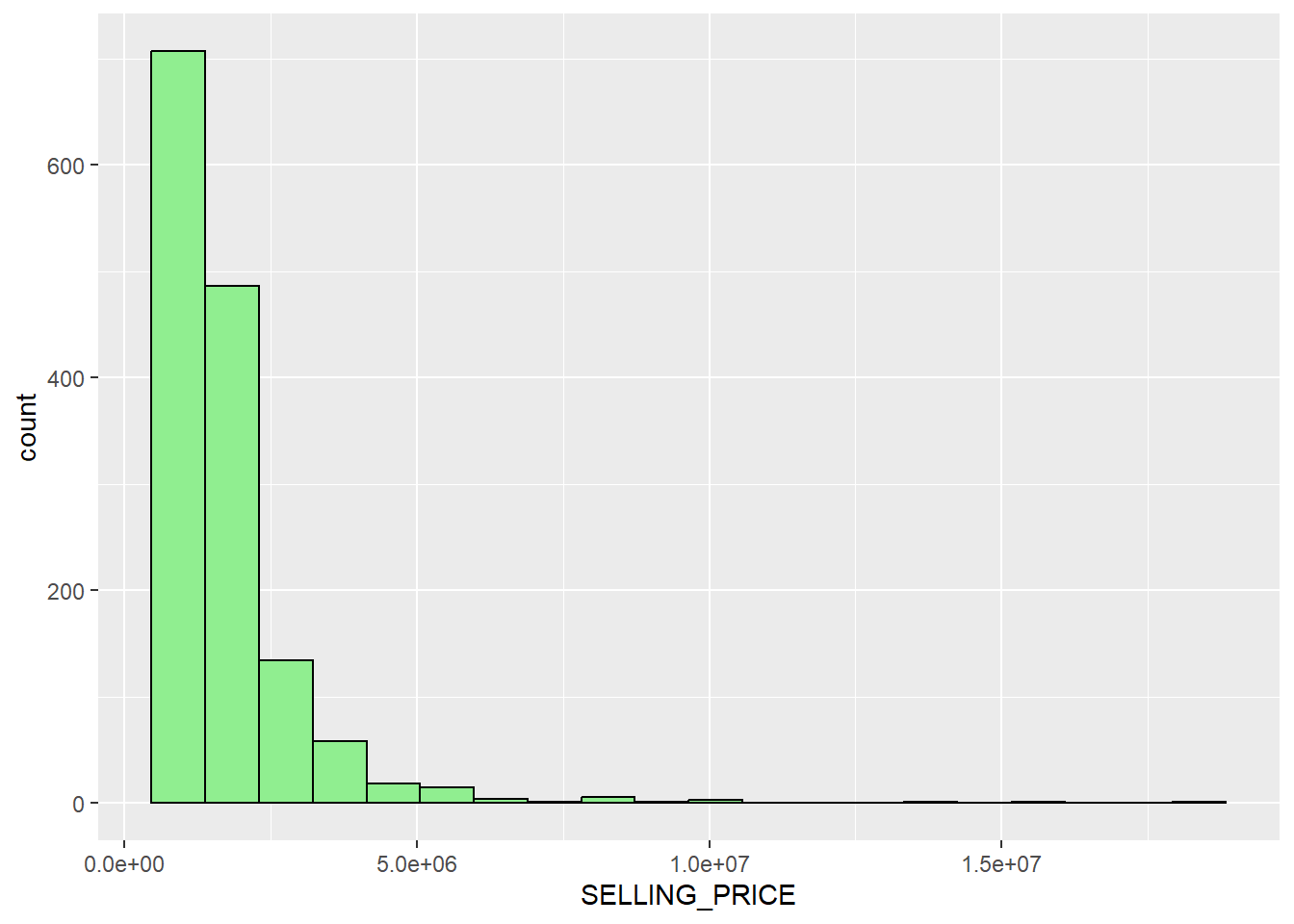
We can observe that the selling price of condo resale apartments shows a right skewed distribution, which can help us conclude that the units were transacted at relatively lower price.
Statistically, we could use Log transformation to normalize the log distribution. It can be achieved by using mutate() of dplyr package.
condo_resale_sf = condo_resale_sf %>%
mutate(`LOG_SELLING_PRICE` = log(SELLING_PRICE))We then plot the histogram of the LOG_SELLING_PRICE as per the code below, the result of the transformation has resulted in a less skewed distribution.
ggplot(data=condo_resale_sf, aes(x=`LOG_SELLING_PRICE`)) +
geom_histogram(bins=20, color="black", fill="light green")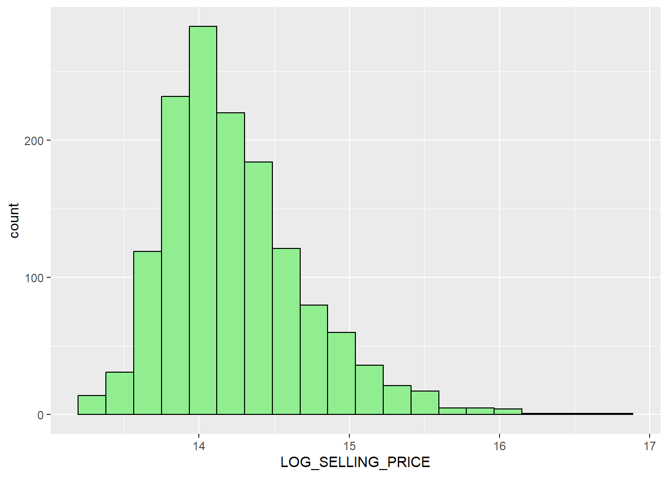
Multiple Histogram Plots distribution of variables
We will learn how to use the ggpubr package’s ggarrange() function to create multiple histogram (also known as a trellis plot) in this part. The 12 histograms are generated using the code snippet below.
AREA_SQM = ggplot(data=condo_resale_sf, aes(x= `AREA_SQM`)) +
geom_histogram(bins=20, color="black", fill="light green")
AGE = ggplot(data=condo_resale_sf, aes(x= `AGE`)) +
geom_histogram(bins=20, color="black", fill="light green")
PROX_CBD = ggplot(data=condo_resale_sf, aes(x= `PROX_CBD`)) +
geom_histogram(bins=20, color="black", fill="light green")
PROX_CHILDCARE = ggplot(data=condo_resale_sf, aes(x= `PROX_CHILDCARE`)) +
geom_histogram(bins=20, color="black", fill="light green")
PROX_ELDERLYCARE = ggplot(data=condo_resale_sf, aes(x= `PROX_ELDERLYCARE`)) +
geom_histogram(bins=20, color="black", fill="light green")
PROX_URA_GROWTH_AREA = ggplot(data=condo_resale_sf,
aes(x= `PROX_URA_GROWTH_AREA`)) +
geom_histogram(bins=20, color="black", fill="light green")
PROX_HAWKER_MARKET = ggplot(data=condo_resale_sf, aes(x= `PROX_HAWKER_MARKET`)) +
geom_histogram(bins=20, color="black", fill="light green")
PROX_KINDERGARTEN = ggplot(data=condo_resale_sf, aes(x= `PROX_KINDERGARTEN`)) +
geom_histogram(bins=20, color="black", fill="light green")
PROX_MRT = ggplot(data=condo_resale_sf, aes(x= `PROX_MRT`)) +
geom_histogram(bins=20, color="black", fill="light green")
PROX_PARK = ggplot(data=condo_resale_sf, aes(x= `PROX_PARK`)) +
geom_histogram(bins=20, color="black", fill="light green")
PROX_PRIMARY_SCH = ggplot(data=condo_resale_sf, aes(x= `PROX_PRIMARY_SCH`)) +
geom_histogram(bins=20, color="black", fill="light green")
PROX_TOP_PRIMARY_SCH = ggplot(data=condo_resale_sf,
aes(x= `PROX_TOP_PRIMARY_SCH`)) +
geom_histogram(bins=20, color="black", fill="light green")
ggarrange(AREA_SQM, AGE, PROX_CBD, PROX_CHILDCARE, PROX_ELDERLYCARE,
PROX_URA_GROWTH_AREA, PROX_HAWKER_MARKET, PROX_KINDERGARTEN, PROX_MRT,
PROX_PARK, PROX_PRIMARY_SCH, PROX_TOP_PRIMARY_SCH,
ncol = 3, nrow = 4)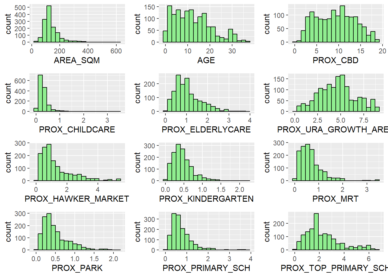
Drawing Statistical Point Map
Lastly, we want to reveal the geospatial distribution condominium resale prices in Singapore. The map will be prepared by using tmap package.
We will turn on the interactive mode of tmap by using the ttm().
There may be issues with the map after reprojection, so we will set tmap_options(check.and.fix = TRUE)
The number of Plan Area N is 55, however the default number of categories is only 30, so we will also need to update it by using tmap_options(max.categories = 55) such that all planning zones are shown
ttm() #tmap_mode("view") #alternative
tmap_options(check.and.fix = TRUE)
tmap_options(max.categories = 55)We then create an interactive symbol map. The tm view() function’s set.zoom.limits argument specifies a minimum and maximum zoom level of 11 and 14, respectively.
tm_shape(mpsz_svy21) +
tm_polygons("PLN_AREA_N") +
tm_shape(condo_resale_sf) +
tm_dots(col = "SELLING_PRICE",
alpha = 0.6,
style="quantile") +
tm_view(set.zoom.limits = c(11,14))ttm() will be used to switch R toggle back tmap back to plot mode before proceeding on to the following section.
ttm()
#tmap_mode("plot") #alternativeHedonic Pricing Modelling in R
In this section, we will learn how to develop Hedonic pricing models for condominium resale units using lm() of R base.
condo_slr = lm(formula = SELLING_PRICE ~ AREA_SQM, data = condo_resale_sf)lm() returns an object of class “lm” or for multiple responses of class c("mlm", "lm").
To acquire and print a summary and analysis of variance table of the results, we can use the functions summary() and anova(). The generic accessor functions coefficients, effects, fitted.values, and residuals take the value returned by lm and extract a number of important properties.
summary(condo_slr)
Call:
lm(formula = SELLING_PRICE ~ AREA_SQM, data = condo_resale_sf)
Residuals:
Min 1Q Median 3Q Max
-3695815 -391764 -87517 258900 13503875
Coefficients:
Estimate Std. Error t value Pr(>|t|)
(Intercept) -258121.1 63517.2 -4.064 5.09e-05 ***
AREA_SQM 14719.0 428.1 34.381 < 2e-16 ***
---
Signif. codes: 0 '***' 0.001 '**' 0.01 '*' 0.05 '.' 0.1 ' ' 1
Residual standard error: 942700 on 1434 degrees of freedom
Multiple R-squared: 0.4518, Adjusted R-squared: 0.4515
F-statistic: 1182 on 1 and 1434 DF, p-value: < 2.2e-16The output report reveals that the SELLING_PRICE can be explained by using the formula:
\[y = - 258121.1 + 14719.0x\]An estimated 45% of the resale prices may be explained by the basic regression model, according to the R-squared value of 0.4518.
We will reject the null hypothesis that mean is a good estimator of SELLING PRICE because the p-value is substantially lower than 0.0001.
Hence, we can conclude that basic linear regression model is a reliable predictor of SELLING_PRICE.
The estimations of the Intercept and AREA SQM both have p-values that are less than 0.001, according to the report’s Coefficients section.
The null hypothesis that B0 and B1 are equal to 0 will therefore be rejected. As a consequence, we can conclude that B0 and B1 are accurate parameter estimates.
To visualise the best fit curve on a scatterplot, we can incorporate lm() as a method function in ggplot’s geometry with the code below.
ggplot(data=condo_resale_sf,
aes(x=`AREA_SQM`, y=`SELLING_PRICE`)) +
geom_point() +
geom_smooth(method = lm)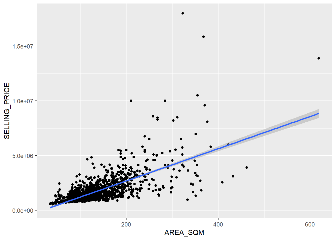
We can observe from the scatter plot that there are a few statistical outliers with relative high selling price
Multiple Linear Regression Method
Visualising the relationships of the independent variables
It’s crucial to make sure that the independent variables employed are not highly correlated with one another before creating a multiple regression model.
The quality of the model will be compromised if these highly correlated independent variables are unintentionally employed in the construction of a multi linear regression model.
In statistics, this phenomenon is referred to as multicollinearity.
Correlation matrix is commonly used to visualize the relationships between the independent variables. Beside the pairs() of R, there are many packages support the display of a correlation matrix. In this section, the corrplot package will be used. We will only be interested in the columns between 5 and 23
corrplot(cor(condo_resale[, 5:23]), diag = FALSE, order = "AOE",
tl.pos = "td", tl.cex = 0.5, method = "number", type = "upper")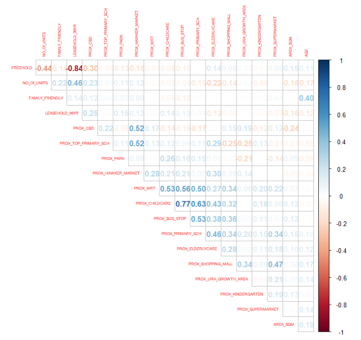
Rearranging the matrix is crucial for uncovering its hidden patterns and structures. Corrplot (parameter order) has four techniques with the names “AOE,” “FPC,” “hclust,” and “alphabet.”
AOE order is applied in the following code section. It uses Michael Friendly’s recommended method of employing the angular order of the eigenvectors to organize the variables.
According to Calkins (2005), variables that can be regarded as having a high degree of correlation are indicated by correlation coefficients with magnitudes between ± 0.7 and 1.0.
From the scatterplot matrix, it is clear that
FREEHOLD is highly correlated to LEASE_99YEAR.
PROX_CHILDCARE is highly correlated to PROX_BUS_STOP.
In view of this, we will exclude LEASE_99YEAR and PROX_CHILDCARE in the subsequent model building.
Building a Hedonic pricing model using multiple linear regression method
The code below using lm() to calibrate the multiple linear regression model.
condo_mlr = lm(formula = SELLING_PRICE ~ AREA_SQM + AGE +
PROX_CBD + PROX_CHILDCARE + PROX_ELDERLYCARE +
PROX_URA_GROWTH_AREA + PROX_HAWKER_MARKET + PROX_KINDERGARTEN +
PROX_MRT + PROX_PARK + PROX_PRIMARY_SCH +
PROX_TOP_PRIMARY_SCH + PROX_SHOPPING_MALL + PROX_SUPERMARKET +
NO_Of_UNITS + FAMILY_FRIENDLY + FREEHOLD,
data=condo_resale_sf)
summary(condo_mlr)
Call:
lm(formula = SELLING_PRICE ~ AREA_SQM + AGE + PROX_CBD + PROX_CHILDCARE +
PROX_ELDERLYCARE + PROX_URA_GROWTH_AREA + PROX_HAWKER_MARKET +
PROX_KINDERGARTEN + PROX_MRT + PROX_PARK + PROX_PRIMARY_SCH +
PROX_TOP_PRIMARY_SCH + PROX_SHOPPING_MALL + PROX_SUPERMARKET +
NO_Of_UNITS + FAMILY_FRIENDLY + FREEHOLD, data = condo_resale_sf)
Residuals:
Min 1Q Median 3Q Max
-3590540 -281747 -24477 246745 12306295
Coefficients:
Estimate Std. Error t value Pr(>|t|)
(Intercept) 510917.15 122292.89 4.178 3.12e-05 ***
AREA_SQM 12792.74 372.23 34.368 < 2e-16 ***
AGE -23742.06 2782.19 -8.534 < 2e-16 ***
PROX_CBD -83603.80 6749.77 -12.386 < 2e-16 ***
PROX_CHILDCARE -71143.44 94343.33 -0.754 0.450920
PROX_ELDERLYCARE 182916.42 42386.79 4.315 1.70e-05 ***
PROX_URA_GROWTH_AREA 35350.01 12610.26 2.803 0.005128 **
PROX_HAWKER_MARKET 34735.30 29454.96 1.179 0.238489
PROX_KINDERGARTEN 111216.65 83018.20 1.340 0.180569
PROX_MRT -238978.09 56345.63 -4.241 2.37e-05 ***
PROX_PARK 542225.90 66960.19 8.098 1.19e-15 ***
PROX_PRIMARY_SCH 188123.51 65753.58 2.861 0.004284 **
PROX_TOP_PRIMARY_SCH 4060.96 20574.79 0.197 0.843562
PROX_SHOPPING_MALL -157419.04 42008.44 -3.747 0.000186 ***
PROX_SUPERMARKET -110417.96 76558.58 -1.442 0.149448
NO_Of_UNITS -212.86 89.69 -2.373 0.017758 *
FAMILY_FRIENDLY 112099.45 47054.54 2.382 0.017335 *
FREEHOLD 328578.90 49210.12 6.677 3.49e-11 ***
---
Signif. codes: 0 '***' 0.001 '**' 0.01 '*' 0.05 '.' 0.1 ' ' 1
Residual standard error: 762000 on 1418 degrees of freedom
Multiple R-squared: 0.6458, Adjusted R-squared: 0.6415
F-statistic: 152.1 on 17 and 1418 DF, p-value: < 2.2e-16Preparing Publication Quality Table: olsrr method
With reference to the summary statistics of condo_mlr, it is clear that not all the independent variables are statistically significant. We will revised the model by removing the variables which are not.
We will then use the ols_regress() function to create the model
condo_mlr1 = lm(formula = SELLING_PRICE ~ AREA_SQM + AGE +
PROX_CBD + PROX_CHILDCARE + PROX_ELDERLYCARE +
PROX_URA_GROWTH_AREA + PROX_MRT + PROX_PARK +
PROX_PRIMARY_SCH + PROX_SHOPPING_MALL +
NO_Of_UNITS + FAMILY_FRIENDLY + FREEHOLD,
data=condo_resale_sf)
ols_regress(condo_mlr1) Model Summary
------------------------------------------------------------------------
R 0.803 RMSE 762505.704
R-Squared 0.644 Coef. Var 43.542
Adj. R-Squared 0.641 MSE 581414949078.040
Pred R-Squared 0.632 MAE 416470.144
------------------------------------------------------------------------
RMSE: Root Mean Square Error
MSE: Mean Square Error
MAE: Mean Absolute Error
ANOVA
--------------------------------------------------------------------------------
Sum of
Squares DF Mean Square F Sig.
--------------------------------------------------------------------------------
Regression 1.497875e+15 13 1.152211e+14 198.174 0.0000
Residual 8.267721e+14 1422 581414949078.040
Total 2.324647e+15 1435
--------------------------------------------------------------------------------
Parameter Estimates
-----------------------------------------------------------------------------------------------------------------
model Beta Std. Error Std. Beta t Sig lower upper
-----------------------------------------------------------------------------------------------------------------
(Intercept) 519269.367 109107.682 4.759 0.000 305240.066 733298.668
AREA_SQM 12855.123 370.341 0.587 34.712 0.000 12128.649 13581.597
AGE -24165.851 2776.771 -0.164 -8.703 0.000 -29612.858 -18718.844
PROX_CBD -80585.330 5772.349 -0.275 -13.961 0.000 -91908.565 -69262.096
PROX_CHILDCARE -15938.701 90778.470 -0.004 -0.176 0.861 -194012.802 162135.399
PROX_ELDERLYCARE 202711.249 40103.083 0.098 5.055 0.000 124043.692 281378.807
PROX_URA_GROWTH_AREA 37328.669 11851.044 0.057 3.150 0.002 14081.263 60576.075
PROX_MRT -220400.480 55474.283 -0.084 -3.973 0.000 -329220.701 -111580.259
PROX_PARK 561964.278 66052.660 0.148 8.508 0.000 432393.157 691535.398
PROX_PRIMARY_SCH 148324.081 60713.107 0.057 2.443 0.015 29227.208 267420.953
PROX_SHOPPING_MALL -189783.935 36354.439 -0.099 -5.220 0.000 -261098.026 -118469.844
NO_Of_UNITS -232.943 88.673 -0.050 -2.627 0.009 -406.887 -58.998
FAMILY_FRIENDLY 118218.279 46968.434 0.046 2.517 0.012 26083.419 210353.139
FREEHOLD 318802.330 48516.584 0.124 6.571 0.000 223630.566 413974.094
-----------------------------------------------------------------------------------------------------------------Looking at the model summary of the report: An estimated 64% of the resale prices may be explained by the multi linear regression model, according to the R-squared value of 0.641.
The null hypothesis is that there is no relationship between the X variables (our parameter estimates in the above report) and the Y variable (the condo resale price).
From the ANOVA analysis, the p-value is highly significant, and hence we will reject the null hypothesis, and can conclude that our parameter estimates variables are accurate.
From the Parameter estimates of the report, the variable PROX_CHILDCARE is not statistically significant as it has a p-value of more than 0.05, thus we will not take this variable into consideration.
With that we can derive our formula as follows:
\[ y = 519269.367 + 12855.123x_1 - 24165.851x_2 - 80585.330x_3 + 202711.249x_4 + 37328.669x_5 - 220400.480x_6 + 561964.278 x_7 + 148324.081x_8 - 189783.935x_9 - 232.943x_{10} + 118218.279x_{11} + 318802.330x_{12} \]
\(x_1\) = AREA_SQM, \(x_2\) = AGE, \(x_3\) = PROX_CBD, \(x_4\) = PROX_ELDERLYCARE, \(x_5\) = PROX_URA_GROWTH_AREA, \(x_6\) = PROX_MRT, \(x_7\) = PROX_PARK, \(x_8\) = PROX_PRIMARY_SCH, \(x_9\) = PROX_SHOPPING_MALL, \(x_{10}\) = NO_Of_UNITS, \(x_{11}\) = FAMILY_FRIENDLY, \(x_{12}\) = FREEHOLD
From the above, we can conclude that the following 7 variables are positive correlated with the condo resale price (i.e. they tend to move in the same direction) - AREA_SQM, PROX_ELDERLYCARE, PROX_URA_GROWTH_AREA, PROX_PARK, PROX_PRIMARY_SCH, FAMILY_FRIENDLY, FREEHOLD
From the above, we can conclude that the following 5 variables are negatively correlated with the condo resale price (i.e. they tend to move in the opposite direction) - AGE, PROX_CBD, PROX_MRT, PROX_SHOPPING_MALL, NO_Of_UNITS
Preparing Publication Quality Table: gtsummary method
An elegant and flexible method for producing publication-quality summary tables in R is the gtsummary package. The tbl_regression() function is used to generate a nicely prepared regression report using the code below.
tbl_regression(condo_mlr1, intercept = TRUE)| Characteristic | Beta | 95% CI1 | p-value |
|---|---|---|---|
| (Intercept) | 519,269 | 305,240, 733,299 | <0.001 |
| AREA_SQM | 12,855 | 12,129, 13,582 | <0.001 |
| AGE | -24,166 | -29,613, -18,719 | <0.001 |
| PROX_CBD | -80,585 | -91,909, -69,262 | <0.001 |
| PROX_CHILDCARE | -15,939 | -194,013, 162,135 | 0.9 |
| PROX_ELDERLYCARE | 202,711 | 124,044, 281,379 | <0.001 |
| PROX_URA_GROWTH_AREA | 37,329 | 14,081, 60,576 | 0.002 |
| PROX_MRT | -220,400 | -329,221, -111,580 | <0.001 |
| PROX_PARK | 561,964 | 432,393, 691,535 | <0.001 |
| PROX_PRIMARY_SCH | 148,324 | 29,227, 267,421 | 0.015 |
| PROX_SHOPPING_MALL | -189,784 | -261,098, -118,470 | <0.001 |
| NO_Of_UNITS | -233 | -407, -59 | 0.009 |
| FAMILY_FRIENDLY | 118,218 | 26,083, 210,353 | 0.012 |
| FREEHOLD | 318,802 | 223,631, 413,974 | <0.001 |
| 1 CI = Confidence Interval | |||
Model statistics can be added to the report using the gtsummary package by either appending them to the report table with the function add_glance_table() or adding them as a table source note with the function add_glance_source_note(), as demonstrated in the code below.
tbl_regression(condo_mlr, intercept = TRUE) %>%
add_glance_source_note(
label = list(sigma ~ "\U03C3"),
include = c(r.squared, adj.r.squared, AIC, statistic, p.value, sigma)
)| Characteristic | Beta | 95% CI1 | p-value |
|---|---|---|---|
| (Intercept) | 510,917 | 271,023, 750,812 | <0.001 |
| AREA_SQM | 12,793 | 12,063, 13,523 | <0.001 |
| AGE | -23,742 | -29,200, -18,284 | <0.001 |
| PROX_CBD | -83,604 | -96,844, -70,363 | <0.001 |
| PROX_CHILDCARE | -71,143 | -256,211, 113,924 | 0.5 |
| PROX_ELDERLYCARE | 182,916 | 99,769, 266,064 | <0.001 |
| PROX_URA_GROWTH_AREA | 35,350 | 10,613, 60,087 | 0.005 |
| PROX_HAWKER_MARKET | 34,735 | -23,045, 92,515 | 0.2 |
| PROX_KINDERGARTEN | 111,217 | -51,635, 274,068 | 0.2 |
| PROX_MRT | -238,978 | -349,508, -128,448 | <0.001 |
| PROX_PARK | 542,226 | 410,874, 673,578 | <0.001 |
| PROX_PRIMARY_SCH | 188,124 | 59,139, 317,108 | 0.004 |
| PROX_TOP_PRIMARY_SCH | 4,061 | -36,299, 44,421 | 0.8 |
| PROX_SHOPPING_MALL | -157,419 | -239,824, -75,014 | <0.001 |
| PROX_SUPERMARKET | -110,418 | -260,598, 39,762 | 0.15 |
| NO_Of_UNITS | -213 | -389, -37 | 0.018 |
| FAMILY_FRIENDLY | 112,099 | 19,795, 204,403 | 0.017 |
| FREEHOLD | 328,579 | 232,046, 425,111 | <0.001 |
| R² = 0.646; Adjusted R² = 0.642; AIC = 42,993; Statistic = 152; p-value = <0.001; σ = 762,022 | |||
| 1 CI = Confidence Interval | |||
For more customization options, refer to Tutorial: tbl_regression
Checking for multicolinearity
A superb R package designed specifically for OLS regression is being introduced in this section. It is known as olsrr. It offers a selection of really helpful techniques for improving multiple linear regression models, including:
comprehensive regression output
residual diagnostics
measures of influence
heteroskedasticity tests
collinearity diagnostics
model fit assessment
variable contribution assessment
variable selection procedures
In the code below, the ols_vif_tol() of olsrr package is used to test if there are sign of multicollinearity.
ols_vif_tol(condo_mlr1) Variables Tolerance VIF
1 AREA_SQM 0.8743701 1.143681
2 AGE 0.7081147 1.412201
3 PROX_CBD 0.6446091 1.551328
4 PROX_CHILDCARE 0.4411869 2.266613
5 PROX_ELDERLYCARE 0.6646092 1.504644
6 PROX_URA_GROWTH_AREA 0.7517424 1.330243
7 PROX_MRT 0.5607764 1.783242
8 PROX_PARK 0.8284731 1.207040
9 PROX_PRIMARY_SCH 0.4531080 2.206979
10 PROX_SHOPPING_MALL 0.6934496 1.442066
11 NO_Of_UNITS 0.6906489 1.447914
12 FAMILY_FRIENDLY 0.7346556 1.361182
13 FREEHOLD 0.7048829 1.418675From the result, the independent variables’ VIF are smaller than 10, therefore, It is safe to conclude that none of the independent variables show any evidence of multicollinearity.
Test for Non-Linearity
It is pertinent to verify the linearity and additivity of the relationship between the dependent and independent variables in multiple linear regression.
In the code below, the ols_plot_resid_fit() function of olsrr package is used to conduct the linearity assumption test.
ols_plot_resid_fit(condo_mlr1)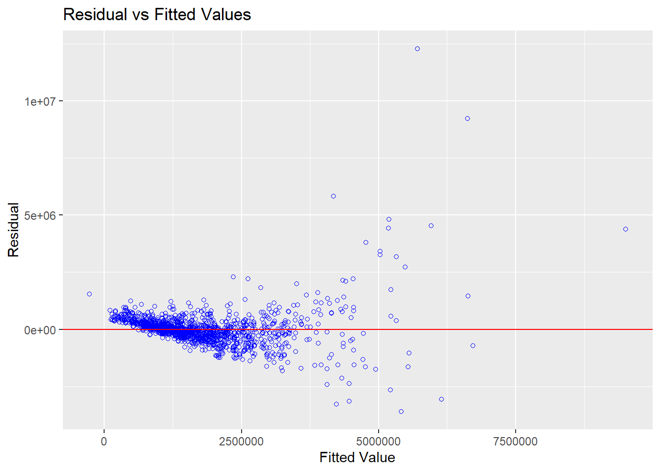
Since the majority of the data points are clustered around the 0 line in the resultant graph above, we can confidently infer that the dependent variable and independent variables have linear relationships.
Test for Normality Assumption
Before doing certain statistical tests or regression, you should ensure that the data generally matches a bell-shaped curve. This is known as the assumption of normality.
The code below uses ols_plot_resid_hist() of olsrr package to perform the normality assumption test.
ols_plot_resid_hist(condo_mlr1)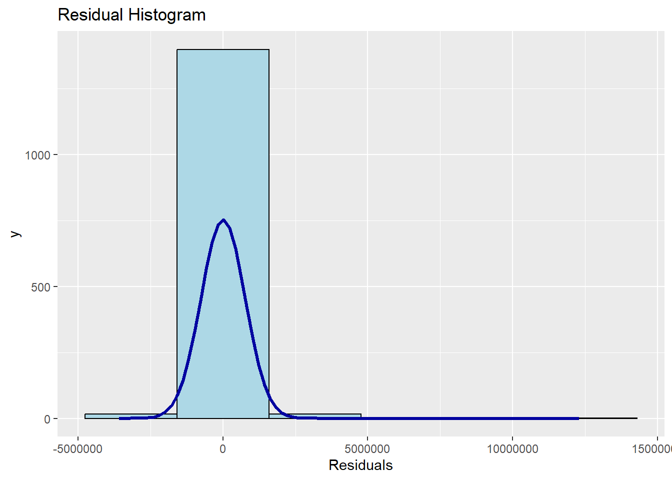
The result shows that the residual of the multiple linear regression model (i.e. condo_mlr1) matches a normal distribution. As demonstrated in the code below, the ols_test_normality() function of the olsrr package can be used if one prefer formal statistical test methods.
ols_test_normality(condo_mlr1)-----------------------------------------------
Test Statistic pvalue
-----------------------------------------------
Shapiro-Wilk 0.6824 0.0000
Kolmogorov-Smirnov 0.1497 0.0000
Cramer-von Mises 120.6722 0.0000
Anderson-Darling 70.7708 0.0000
-----------------------------------------------The p-values for the four tests are less than the alpha value of 0.05, as shown in the summary table above. Therefore, we will conclude that the residuals are not normally distributed and reject the null hypothesis.
Testing for Spatial Autocorrelation
Since the Hedonic model we attempt to construct uses attributes that are geographically referenced, it is important for us to see the residual of the Hedonic pricing model.
condo_resale_sf from the SF data frame needs to be transformed into a SpatialPointsDataFrame in order to run the spatial autocorrelation test.
First, export the residual of the Hedonic pricing model and save it as a data frame using
as.data.frame()mlr_output = as.data.frame(condo_mlr1$residuals)Join the newly created data frame with condo_resale_sf object with
cbind().condo_resale_res_sf = cbind(condo_resale_sf, mlr_output) %>% rename(`MLR_RES` = `condo_mlr1.residuals`)Because the spdep package can only process sp compliant spatial data objects, we need to transform condo_resale_res_sf from a simple feature object into a SpatialPointsDataFrame with
as_spatial()condo_resale_sp = as_Spatial(condo_resale_res_sf)We will use tmap package to display the distribution of the residuals on an interactive map
ttm() symbolmap = tm_shape(mpsz_svy21) + tmap_options(check.and.fix = TRUE) + tm_polygons("PLN_AREA_N", alpha = 0.5) + tm_shape(condo_resale_res_sf) + tm_dots(col = "MLR_RES", alpha = 0.8, style="quantile") + tm_view(set.zoom.limits = c(11,14)) symbolmapttm()
There are indications of spatial autocorrelation, as shown by the map above. The Moran’s I test can be use to verify if our observation is accurate.
Moran’s I test for spatial autocorrelation
We will create the distance base matrix by using dnearneigh() function of spdep.
nb = dnearneigh(coordinates(condo_resale_sp), 0, 1500, longlat = FALSE)
summary(nb)Neighbour list object:
Number of regions: 1436
Number of nonzero links: 66266
Percentage nonzero weights: 3.213526
Average number of links: 46.14624
Link number distribution:
1 3 5 7 9 10 11 12 13 14 15 16 17 18 19 20 21 22 23 24
3 3 9 4 3 15 10 19 17 45 19 5 14 29 19 6 35 45 18 47
25 26 27 28 29 30 31 32 33 34 35 36 37 38 39 40 41 42 43 44
16 43 22 26 21 11 9 23 22 13 16 25 21 37 16 18 8 21 4 12
45 46 47 48 49 50 51 52 53 54 55 56 57 58 59 60 61 62 63 64
8 36 18 14 14 43 11 12 8 13 12 13 4 5 6 12 11 20 29 33
65 66 67 68 69 70 71 72 73 74 75 76 77 78 79 80 81 82 83 84
15 20 10 14 15 15 11 16 12 10 8 19 12 14 9 8 4 13 11 6
85 86 87 88 89 90 91 92 93 94 95 96 97 98 99 100 101 102 103 104
4 9 4 4 4 6 2 16 9 4 5 9 3 9 4 2 1 2 1 1
105 106 107 108 109 110 112 116 125
1 5 9 2 1 3 1 1 1
3 least connected regions:
193 194 277 with 1 link
1 most connected region:
285 with 125 linksThe resulting neighbours lists (nb) will then be transformed into spatial weights using the nb2listw() function of the spdep packge.
nb_lw = nb2listw(nb, style = 'W')
summary(nb_lw)Characteristics of weights list object:
Neighbour list object:
Number of regions: 1436
Number of nonzero links: 66266
Percentage nonzero weights: 3.213526
Average number of links: 46.14624
Link number distribution:
1 3 5 7 9 10 11 12 13 14 15 16 17 18 19 20 21 22 23 24
3 3 9 4 3 15 10 19 17 45 19 5 14 29 19 6 35 45 18 47
25 26 27 28 29 30 31 32 33 34 35 36 37 38 39 40 41 42 43 44
16 43 22 26 21 11 9 23 22 13 16 25 21 37 16 18 8 21 4 12
45 46 47 48 49 50 51 52 53 54 55 56 57 58 59 60 61 62 63 64
8 36 18 14 14 43 11 12 8 13 12 13 4 5 6 12 11 20 29 33
65 66 67 68 69 70 71 72 73 74 75 76 77 78 79 80 81 82 83 84
15 20 10 14 15 15 11 16 12 10 8 19 12 14 9 8 4 13 11 6
85 86 87 88 89 90 91 92 93 94 95 96 97 98 99 100 101 102 103 104
4 9 4 4 4 6 2 16 9 4 5 9 3 9 4 2 1 2 1 1
105 106 107 108 109 110 112 116 125
1 5 9 2 1 3 1 1 1
3 least connected regions:
193 194 277 with 1 link
1 most connected region:
285 with 125 links
Weights style: W
Weights constants summary:
n nn S0 S1 S2
W 1436 2062096 1436 94.81916 5798.341The null hypothesis
The null hypothesis in this case is that residuals are randomly distributed.
lm.morantest() of spdep package will be used to perform Moran’s I test for residual spatial autocorrelation
lm.morantest(condo_mlr1, nb_lw)
Global Moran I for regression residuals
data:
model: lm(formula = SELLING_PRICE ~ AREA_SQM + AGE + PROX_CBD +
PROX_CHILDCARE + PROX_ELDERLYCARE + PROX_URA_GROWTH_AREA + PROX_MRT +
PROX_PARK + PROX_PRIMARY_SCH + PROX_SHOPPING_MALL + NO_Of_UNITS +
FAMILY_FRIENDLY + FREEHOLD, data = condo_resale_sf)
weights: nb_lw
Moran I statistic standard deviate = 25.153, p-value < 2.2e-16
alternative hypothesis: greater
sample estimates:
Observed Moran I Expectation Variance
1.501510e-01 -5.172738e-03 3.813245e-05 Based on the result, we will reject the null hypothesis as the p-value is less than 0.05. In fact as the p-value is less than 0.01, we can consider that as highly significant.
Therefore, we can conclude that the residuals is not randomly distributed based on Moran’s I statistics.
As the observed Global Moran I is 0.1438876, which is more than 0, we can then also conclude that the residuals follows a cluster distribution.
Building Hedonic Pricing Models using GW model
We will be introduced to model Hedonic pricing in this section using both fixed and adaptive bandwidth strategies.
Building Fixed Bandwidth GWR Model
Computing Fixed Bandwidth
The optimal fixed bandwidth to employ in the model is chosen using the bw.gwr() function of the GWModel package, which is utilized in the code block below.
The argument adaptive is set to FALSE, indicating that we want to compute the fixed bandwidth
The CV cross-validation approach and the AIC corrected (AICc) approach are the two methods that could be used to identify the stopping rule. We use the approach argument to define the stopping rule.
CV cross-validation Approach - FIXED Bandwidth
bw.fixed.cv = bw.gwr(formula = SELLING_PRICE ~ AREA_SQM + AGE + PROX_CBD + PROX_CHILDCARE + PROX_ELDERLYCARE + PROX_URA_GROWTH_AREA + PROX_MRT + PROX_PARK + PROX_PRIMARY_SCH + PROX_SHOPPING_MALL + NO_Of_UNITS + FAMILY_FRIENDLY + FREEHOLD, data=condo_resale_sp,
approach = "CV",
kernel = "gaussian",
adaptive = FALSE,
longlat = FALSE
)Fixed bandwidth: 17660.96 CV score: 8.38823e+14
Fixed bandwidth: 10917.26 CV score: 8.094681e+14
Fixed bandwidth: 6749.419 CV score: 7.40732e+14
Fixed bandwidth: 4173.553 CV score: 6.444863e+14
Fixed bandwidth: 2581.58 CV score: 5.595032e+14
Fixed bandwidth: 1597.687 CV score: 5.057075e+14
Fixed bandwidth: 989.6077 CV score: 4.90792e+14
Fixed bandwidth: 613.7939 CV score: 2.464871e+16
Fixed bandwidth: 1221.873 CV score: 4.938091e+14
Fixed bandwidth: 846.0596 CV score: 5.039352e+14
Fixed bandwidth: 1078.325 CV score: 4.913612e+14
Fixed bandwidth: 934.7772 CV score: 4.917418e+14
Fixed bandwidth: 1023.495 CV score: 4.9078e+14
Fixed bandwidth: 1044.438 CV score: 4.909375e+14
Fixed bandwidth: 1010.551 CV score: 4.907407e+14
Fixed bandwidth: 1002.551 CV score: 4.907425e+14
Fixed bandwidth: 1015.495 CV score: 4.907498e+14
Fixed bandwidth: 1007.495 CV score: 4.907389e+14
Fixed bandwidth: 1005.607 CV score: 4.907394e+14
Fixed bandwidth: 1008.663 CV score: 4.907393e+14
Fixed bandwidth: 1006.774 CV score: 4.90739e+14
Fixed bandwidth: 1007.941 CV score: 4.90739e+14
Fixed bandwidth: 1007.22 CV score: 4.907389e+14
Fixed bandwidth: 1007.05 CV score: 4.907389e+14
Fixed bandwidth: 1007.325 CV score: 4.907389e+14
Fixed bandwidth: 1007.155 CV score: 4.907389e+14
Fixed bandwidth: 1007.26 CV score: 4.907389e+14
Fixed bandwidth: 1007.195 CV score: 4.907389e+14
Fixed bandwidth: 1007.235 CV score: 4.907389e+14
Fixed bandwidth: 1007.245 CV score: 4.907389e+14
Fixed bandwidth: 1007.229 CV score: 4.907389e+14
Fixed bandwidth: 1007.226 CV score: 4.907389e+14
Fixed bandwidth: 1007.232 CV score: 4.907389e+14
Fixed bandwidth: 1007.228 CV score: 4.907389e+14
Fixed bandwidth: 1007.23 CV score: 4.907389e+14
Fixed bandwidth: 1007.229 CV score: 4.907389e+14
Fixed bandwidth: 1007.23 CV score: 4.907389e+14
Fixed bandwidth: 1007.229 CV score: 4.907389e+14
Fixed bandwidth: 1007.23 CV score: 4.907389e+14
Fixed bandwidth: 1007.229 CV score: 4.907389e+14
Fixed bandwidth: 1007.229 CV score: 4.907389e+14
Fixed bandwidth: 1007.229 CV score: 4.907389e+14 The result shows that the recommended bandwidth is 1007.229 metres. The reason why it is in meters is due to the fact that the projection system SYV21 measures distance in meters.
GWModel method - CV cross-validation Approach - FIXED Bandwidth
Now, utilizing fixed bandwidth and a Gaussian kernel, we may calibrate the gwr model using the code below.
gwr.fixed.cv = gwr.basic(formula = SELLING_PRICE ~ AREA_SQM + AGE + PROX_CBD + PROX_CHILDCARE + PROX_ELDERLYCARE + PROX_URA_GROWTH_AREA + PROX_MRT + PROX_PARK + PROX_PRIMARY_SCH + PROX_SHOPPING_MALL + NO_Of_UNITS + FAMILY_FRIENDLY + FREEHOLD,
data=condo_resale_sp,
bw=bw.fixed.cv,
kernel = "gaussian",
longlat = FALSE
)
gwr.fixed.cv ***********************************************************************
* Package GWmodel *
***********************************************************************
Program starts at: 2023-01-10 00:45:41
Call:
gwr.basic(formula = SELLING_PRICE ~ AREA_SQM + AGE + PROX_CBD +
PROX_CHILDCARE + PROX_ELDERLYCARE + PROX_URA_GROWTH_AREA +
PROX_MRT + PROX_PARK + PROX_PRIMARY_SCH + PROX_SHOPPING_MALL +
NO_Of_UNITS + FAMILY_FRIENDLY + FREEHOLD, data = condo_resale_sp,
bw = bw.fixed.cv, kernel = "gaussian", longlat = FALSE)
Dependent (y) variable: SELLING_PRICE
Independent variables: AREA_SQM AGE PROX_CBD PROX_CHILDCARE PROX_ELDERLYCARE PROX_URA_GROWTH_AREA PROX_MRT PROX_PARK PROX_PRIMARY_SCH PROX_SHOPPING_MALL NO_Of_UNITS FAMILY_FRIENDLY FREEHOLD
Number of data points: 1436
***********************************************************************
* Results of Global Regression *
***********************************************************************
Call:
lm(formula = formula, data = data)
Residuals:
Min 1Q Median 3Q Max
-3590706 -278747 -27795 255777 12287214
Coefficients:
Estimate Std. Error t value Pr(>|t|)
(Intercept) 519269.37 109107.68 4.759 2.14e-06 ***
AREA_SQM 12855.12 370.34 34.712 < 2e-16 ***
AGE -24165.85 2776.77 -8.703 < 2e-16 ***
PROX_CBD -80585.33 5772.35 -13.961 < 2e-16 ***
PROX_CHILDCARE -15938.70 90778.47 -0.176 0.86065
PROX_ELDERLYCARE 202711.25 40103.08 5.055 4.87e-07 ***
PROX_URA_GROWTH_AREA 37328.67 11851.04 3.150 0.00167 **
PROX_MRT -220400.48 55474.28 -3.973 7.45e-05 ***
PROX_PARK 561964.28 66052.66 8.508 < 2e-16 ***
PROX_PRIMARY_SCH 148324.08 60713.11 2.443 0.01469 *
PROX_SHOPPING_MALL -189783.94 36354.44 -5.220 2.05e-07 ***
NO_Of_UNITS -232.94 88.67 -2.627 0.00871 **
FAMILY_FRIENDLY 118218.28 46968.43 2.517 0.01195 *
FREEHOLD 318802.33 48516.58 6.571 6.99e-11 ***
---Significance stars
Signif. codes: 0 '***' 0.001 '**' 0.01 '*' 0.05 '.' 0.1 ' ' 1
Residual standard error: 762500 on 1422 degrees of freedom
Multiple R-squared: 0.6443
Adjusted R-squared: 0.6411
F-statistic: 198.2 on 13 and 1422 DF, p-value: < 2.2e-16
***Extra Diagnostic information
Residual sum of squares: 8.267721e+14
Sigma(hat): 759308.6
AIC: 42990.54
AICc: 42990.88
BIC: 41742.63
***********************************************************************
* Results of Geographically Weighted Regression *
***********************************************************************
*********************Model calibration information*********************
Kernel function: gaussian
Fixed bandwidth: 1007.229
Regression points: the same locations as observations are used.
Distance metric: Euclidean distance metric is used.
****************Summary of GWR coefficient estimates:******************
Min. 1st Qu. Median 3rd Qu.
Intercept -3.5989e+07 -4.4060e+05 9.2831e+05 1.8466e+06
AREA_SQM 1.1785e+03 5.2340e+03 7.5401e+03 1.2296e+04
AGE -9.7849e+04 -2.0056e+04 -8.3394e+03 -3.3290e+03
PROX_CBD -6.9655e+07 -2.5784e+05 -8.7757e+04 -7.5747e+02
PROX_CHILDCARE -8.0616e+06 -3.1063e+05 -2.8980e+04 3.0356e+05
PROX_ELDERLYCARE -1.8027e+06 -1.0618e+05 7.6538e+04 2.2542e+05
PROX_URA_GROWTH_AREA -2.3792e+06 -6.2508e+04 6.3534e+04 2.3727e+05
PROX_MRT -2.0104e+06 -4.6706e+05 -1.5757e+05 2.1115e+04
PROX_PARK -1.1677e+06 -1.8131e+05 -2.3913e+03 3.6967e+05
PROX_PRIMARY_SCH -7.9643e+06 -2.0448e+05 3.8724e+04 4.9478e+05
PROX_SHOPPING_MALL -3.1354e+06 -1.5589e+05 2.2518e+04 1.9964e+05
NO_Of_UNITS -1.2150e+03 -1.9893e+02 2.3880e+01 2.9194e+02
FAMILY_FRIENDLY -3.4772e+06 -1.0712e+05 9.2370e+03 1.6842e+05
FREEHOLD -2.9216e+06 2.3948e+04 1.4841e+05 3.6382e+05
Max.
Intercept 65653406
AREA_SQM 21460
AGE 216486
PROX_CBD 1840742
PROX_CHILDCARE 1623235
PROX_ELDERLYCARE 22759869
PROX_URA_GROWTH_AREA 70603320
PROX_MRT 1884569
PROX_PARK 17194282
PROX_PRIMARY_SCH 3160858
PROX_SHOPPING_MALL 2663514
NO_Of_UNITS 10138
FAMILY_FRIENDLY 1748670
FREEHOLD 5172108
************************Diagnostic information*************************
Number of data points: 1436
Effective number of parameters (2trace(S) - trace(S'S)): 394.4464
Effective degrees of freedom (n-2trace(S) + trace(S'S)): 1041.554
AICc (GWR book, Fotheringham, et al. 2002, p. 61, eq 2.33): 42298.78
AIC (GWR book, Fotheringham, et al. 2002,GWR p. 96, eq. 4.22): 41764.82
BIC (GWR book, Fotheringham, et al. 2002,GWR p. 61, eq. 2.34): 42405.37
Residual sum of squares: 2.854911e+14
R-square value: 0.8771895
Adjusted R-square value: 0.8306352
***********************************************************************
Program stops at: 2023-01-10 00:45:42 The report shows that the adjusted \(R^2\) of the gwr is 0.8306, which is significantly better than the global multiple linear regression model of 0.6411.
The AICC Value in this case is 42298.78
AIC corrected (AICc) Approach - FIXED Bandwidth
We use the same functionbw.gwr() here, except that we will change the approach to AICc
bw.fixed.aicc = bw.gwr(formula = SELLING_PRICE ~ AREA_SQM + AGE + PROX_CBD + PROX_CHILDCARE + PROX_ELDERLYCARE + PROX_URA_GROWTH_AREA + PROX_MRT + PROX_PARK + PROX_PRIMARY_SCH + PROX_SHOPPING_MALL + NO_Of_UNITS + FAMILY_FRIENDLY + FREEHOLD, data=condo_resale_sp,
approach = "AICc",
kernel = "gaussian",
adaptive = FALSE,
longlat = FALSE
)Fixed bandwidth: 17660.96 AICc value: 42960.36
Fixed bandwidth: 10917.26 AICc value: 42908.6
Fixed bandwidth: 6749.419 AICc value: 42783.31
Fixed bandwidth: 4173.553 AICc value: 42595.92
Fixed bandwidth: 2581.58 AICc value: 42413.44
Fixed bandwidth: 1597.687 AICc value: 42303.87
Fixed bandwidth: 989.6077 AICc value: 42300.54
Fixed bandwidth: 613.7939 AICc value: 42436.47
Fixed bandwidth: 1221.873 AICc value: 42292.04
Fixed bandwidth: 1365.421 AICc value: 42294.49
Fixed bandwidth: 1133.156 AICc value: 42292.45
Fixed bandwidth: 1276.704 AICc value: 42292.63
Fixed bandwidth: 1187.986 AICc value: 42291.96
Fixed bandwidth: 1167.043 AICc value: 42292.04
Fixed bandwidth: 1200.93 AICc value: 42291.96
Fixed bandwidth: 1179.987 AICc value: 42291.98
Fixed bandwidth: 1192.93 AICc value: 42291.95
Fixed bandwidth: 1195.986 AICc value: 42291.95
Fixed bandwidth: 1191.042 AICc value: 42291.96
Fixed bandwidth: 1194.097 AICc value: 42291.95
Fixed bandwidth: 1194.819 AICc value: 42291.95 The result shows that the recommended bandwidth is 1194.819 metres.
GWModel method - AIC corrected (AICc) Approach - FIXED Bandwidth
Now, utilizing fixed bandwidth and a Gaussian kernel, we may calibrate the gwr model using the code below.
gwr.fixed.aicc = gwr.basic(formula = SELLING_PRICE ~ AREA_SQM + AGE + PROX_CBD + PROX_CHILDCARE + PROX_ELDERLYCARE + PROX_URA_GROWTH_AREA + PROX_MRT + PROX_PARK + PROX_PRIMARY_SCH + PROX_SHOPPING_MALL + NO_Of_UNITS + FAMILY_FRIENDLY + FREEHOLD,
data=condo_resale_sp,
bw=bw.fixed.aicc,
kernel = "gaussian",
longlat = FALSE
)
gwr.fixed.aicc ***********************************************************************
* Package GWmodel *
***********************************************************************
Program starts at: 2023-01-10 00:45:54
Call:
gwr.basic(formula = SELLING_PRICE ~ AREA_SQM + AGE + PROX_CBD +
PROX_CHILDCARE + PROX_ELDERLYCARE + PROX_URA_GROWTH_AREA +
PROX_MRT + PROX_PARK + PROX_PRIMARY_SCH + PROX_SHOPPING_MALL +
NO_Of_UNITS + FAMILY_FRIENDLY + FREEHOLD, data = condo_resale_sp,
bw = bw.fixed.aicc, kernel = "gaussian", longlat = FALSE)
Dependent (y) variable: SELLING_PRICE
Independent variables: AREA_SQM AGE PROX_CBD PROX_CHILDCARE PROX_ELDERLYCARE PROX_URA_GROWTH_AREA PROX_MRT PROX_PARK PROX_PRIMARY_SCH PROX_SHOPPING_MALL NO_Of_UNITS FAMILY_FRIENDLY FREEHOLD
Number of data points: 1436
***********************************************************************
* Results of Global Regression *
***********************************************************************
Call:
lm(formula = formula, data = data)
Residuals:
Min 1Q Median 3Q Max
-3590706 -278747 -27795 255777 12287214
Coefficients:
Estimate Std. Error t value Pr(>|t|)
(Intercept) 519269.37 109107.68 4.759 2.14e-06 ***
AREA_SQM 12855.12 370.34 34.712 < 2e-16 ***
AGE -24165.85 2776.77 -8.703 < 2e-16 ***
PROX_CBD -80585.33 5772.35 -13.961 < 2e-16 ***
PROX_CHILDCARE -15938.70 90778.47 -0.176 0.86065
PROX_ELDERLYCARE 202711.25 40103.08 5.055 4.87e-07 ***
PROX_URA_GROWTH_AREA 37328.67 11851.04 3.150 0.00167 **
PROX_MRT -220400.48 55474.28 -3.973 7.45e-05 ***
PROX_PARK 561964.28 66052.66 8.508 < 2e-16 ***
PROX_PRIMARY_SCH 148324.08 60713.11 2.443 0.01469 *
PROX_SHOPPING_MALL -189783.94 36354.44 -5.220 2.05e-07 ***
NO_Of_UNITS -232.94 88.67 -2.627 0.00871 **
FAMILY_FRIENDLY 118218.28 46968.43 2.517 0.01195 *
FREEHOLD 318802.33 48516.58 6.571 6.99e-11 ***
---Significance stars
Signif. codes: 0 '***' 0.001 '**' 0.01 '*' 0.05 '.' 0.1 ' ' 1
Residual standard error: 762500 on 1422 degrees of freedom
Multiple R-squared: 0.6443
Adjusted R-squared: 0.6411
F-statistic: 198.2 on 13 and 1422 DF, p-value: < 2.2e-16
***Extra Diagnostic information
Residual sum of squares: 8.267721e+14
Sigma(hat): 759308.6
AIC: 42990.54
AICc: 42990.88
BIC: 41742.63
***********************************************************************
* Results of Geographically Weighted Regression *
***********************************************************************
*********************Model calibration information*********************
Kernel function: gaussian
Fixed bandwidth: 1194.097
Regression points: the same locations as observations are used.
Distance metric: Euclidean distance metric is used.
****************Summary of GWR coefficient estimates:******************
Min. 1st Qu. Median 3rd Qu.
Intercept -1.3229e+07 -2.5294e+05 1.0715e+06 1.7346e+06
AREA_SQM 2.0405e+03 5.4005e+03 7.6494e+03 1.2453e+04
AGE -8.9281e+04 -1.9578e+04 -8.5466e+03 -4.4587e+03
PROX_CBD -2.0613e+07 -2.1353e+05 -9.5218e+04 -2.3752e+04
PROX_CHILDCARE -4.2233e+06 -2.1408e+05 1.1091e+04 4.0355e+05
PROX_ELDERLYCARE -1.1247e+06 -6.2073e+04 8.2792e+04 2.4482e+05
PROX_URA_GROWTH_AREA -8.4682e+05 -5.1568e+04 5.3971e+04 1.8620e+05
PROX_MRT -1.9291e+06 -4.1052e+05 -1.9356e+05 -6.0160e+04
PROX_PARK -9.8989e+05 -1.5051e+05 1.0306e+04 3.2994e+05
PROX_PRIMARY_SCH -2.9010e+06 -1.3952e+05 2.1568e+04 4.6016e+05
PROX_SHOPPING_MALL -1.2198e+06 -1.1194e+05 1.6117e+04 1.5018e+05
NO_Of_UNITS -1.1290e+03 -2.2506e+02 5.0862e+00 2.0688e+02
FAMILY_FRIENDLY -1.8918e+06 -8.9121e+04 9.8099e+03 1.5753e+05
FREEHOLD -7.3765e+05 5.5294e+04 1.5083e+05 3.6461e+05
Max.
Intercept 4260694.8
AREA_SQM 20492.7
AGE 71586.8
PROX_CBD 708742.7
PROX_CHILDCARE 1777012.3
PROX_ELDERLYCARE 9962633.8
PROX_URA_GROWTH_AREA 21133083.9
PROX_MRT 1489742.3
PROX_PARK 5551558.3
PROX_PRIMARY_SCH 2428052.5
PROX_SHOPPING_MALL 1027750.6
NO_Of_UNITS 3812.8
FAMILY_FRIENDLY 1488223.6
FREEHOLD 1204377.3
************************Diagnostic information*************************
Number of data points: 1436
Effective number of parameters (2trace(S) - trace(S'S)): 331.8507
Effective degrees of freedom (n-2trace(S) + trace(S'S)): 1104.149
AICc (GWR book, Fotheringham, et al. 2002, p. 61, eq 2.33): 42291.95
AIC (GWR book, Fotheringham, et al. 2002,GWR p. 96, eq. 4.22): 41885.25
BIC (GWR book, Fotheringham, et al. 2002,GWR p. 61, eq. 2.34): 42166.64
Residual sum of squares: 3.231014e+14
R-square value: 0.8610105
Adjusted R-square value: 0.8191996
***********************************************************************
Program stops at: 2023-01-10 00:45:55 The report shows that the adjusted \(R^2\) of the gwr is 0.8192, which is significantly better than the global multiple linear regression model of 0.6411.
The AICC Value in this case is 42291.95.
Comparison of the 2 approaches for FIXED Bandwidth
Comparing the AICC value of using the CV Approach (42298.78) vs the AICC Approach (42291.95), the difference between the 2 method differs by 6.83, which is greater than 3. Hence we can conclude that the AICC Approach for fixed bandwidth is a better model
Building Adaptive Bandwidth GWR Model
In this section, we’ll use an adaptive bandwidth approach to calibrate the gwr-based Hedonic pricing model.
Computing the adaptive bandwidth
Similar to the earlier section, we will first use bw.ger() to determine the recommended data point to use.
The code used look very similar to the one used to compute the fixed bandwidth except the adaptive argument has changed to TRUE.
CV cross-validation Approach - ADAPTIVE Bandwidth
bw.adaptive.cv = bw.gwr(formula = SELLING_PRICE ~ AREA_SQM + AGE + PROX_CBD + PROX_CHILDCARE + PROX_ELDERLYCARE + PROX_URA_GROWTH_AREA + PROX_MRT + PROX_PARK + PROX_PRIMARY_SCH + PROX_SHOPPING_MALL + NO_Of_UNITS + FAMILY_FRIENDLY + FREEHOLD,
data=condo_resale_sp,
approach = "CV",
kernel = "gaussian",
adaptive = TRUE,
longlat = FALSE
)Adaptive bandwidth: 895 CV score: 8.083801e+14
Adaptive bandwidth: 561 CV score: 7.795885e+14
Adaptive bandwidth: 354 CV score: 7.070578e+14
Adaptive bandwidth: 226 CV score: 6.318468e+14
Adaptive bandwidth: 147 CV score: 5.866026e+14
Adaptive bandwidth: 98 CV score: 5.602514e+14
Adaptive bandwidth: 68 CV score: 5.343671e+14
Adaptive bandwidth: 49 CV score: 5.050443e+14
Adaptive bandwidth: 37 CV score: 4.897866e+14
Adaptive bandwidth: 30 CV score: 4.693701e+14
Adaptive bandwidth: 25 CV score: 4.713118e+14
Adaptive bandwidth: 32 CV score: 4.785995e+14
Adaptive bandwidth: 27 CV score: 4.745487e+14
Adaptive bandwidth: 30 CV score: 4.693701e+14 The outcome demonstrates that 30 data points should be used.
GWModel method - CV cross-validation Approach - ADAPTIVE Bandwidth
Now, utilizing fixed bandwidth and a Gaussian kernel, we may calibrate the gwr model using the code below.
gwr.adaptive.cv = gwr.basic(formula = SELLING_PRICE ~ AREA_SQM + AGE + PROX_CBD + PROX_CHILDCARE + PROX_ELDERLYCARE +
PROX_URA_GROWTH_AREA + PROX_MRT + PROX_PARK +
PROX_PRIMARY_SCH + PROX_SHOPPING_MALL + NO_Of_UNITS + FAMILY_FRIENDLY + FREEHOLD,
data=condo_resale_sp,
bw=bw.adaptive.cv,
kernel = 'gaussian',
adaptive=TRUE,
longlat = FALSE)
gwr.adaptive.cv ***********************************************************************
* Package GWmodel *
***********************************************************************
Program starts at: 2023-01-10 00:46:01
Call:
gwr.basic(formula = SELLING_PRICE ~ AREA_SQM + AGE + PROX_CBD +
PROX_CHILDCARE + PROX_ELDERLYCARE + PROX_URA_GROWTH_AREA +
PROX_MRT + PROX_PARK + PROX_PRIMARY_SCH + PROX_SHOPPING_MALL +
NO_Of_UNITS + FAMILY_FRIENDLY + FREEHOLD, data = condo_resale_sp,
bw = bw.adaptive.cv, kernel = "gaussian", adaptive = TRUE,
longlat = FALSE)
Dependent (y) variable: SELLING_PRICE
Independent variables: AREA_SQM AGE PROX_CBD PROX_CHILDCARE PROX_ELDERLYCARE PROX_URA_GROWTH_AREA PROX_MRT PROX_PARK PROX_PRIMARY_SCH PROX_SHOPPING_MALL NO_Of_UNITS FAMILY_FRIENDLY FREEHOLD
Number of data points: 1436
***********************************************************************
* Results of Global Regression *
***********************************************************************
Call:
lm(formula = formula, data = data)
Residuals:
Min 1Q Median 3Q Max
-3590706 -278747 -27795 255777 12287214
Coefficients:
Estimate Std. Error t value Pr(>|t|)
(Intercept) 519269.37 109107.68 4.759 2.14e-06 ***
AREA_SQM 12855.12 370.34 34.712 < 2e-16 ***
AGE -24165.85 2776.77 -8.703 < 2e-16 ***
PROX_CBD -80585.33 5772.35 -13.961 < 2e-16 ***
PROX_CHILDCARE -15938.70 90778.47 -0.176 0.86065
PROX_ELDERLYCARE 202711.25 40103.08 5.055 4.87e-07 ***
PROX_URA_GROWTH_AREA 37328.67 11851.04 3.150 0.00167 **
PROX_MRT -220400.48 55474.28 -3.973 7.45e-05 ***
PROX_PARK 561964.28 66052.66 8.508 < 2e-16 ***
PROX_PRIMARY_SCH 148324.08 60713.11 2.443 0.01469 *
PROX_SHOPPING_MALL -189783.94 36354.44 -5.220 2.05e-07 ***
NO_Of_UNITS -232.94 88.67 -2.627 0.00871 **
FAMILY_FRIENDLY 118218.28 46968.43 2.517 0.01195 *
FREEHOLD 318802.33 48516.58 6.571 6.99e-11 ***
---Significance stars
Signif. codes: 0 '***' 0.001 '**' 0.01 '*' 0.05 '.' 0.1 ' ' 1
Residual standard error: 762500 on 1422 degrees of freedom
Multiple R-squared: 0.6443
Adjusted R-squared: 0.6411
F-statistic: 198.2 on 13 and 1422 DF, p-value: < 2.2e-16
***Extra Diagnostic information
Residual sum of squares: 8.267721e+14
Sigma(hat): 759308.6
AIC: 42990.54
AICc: 42990.88
BIC: 41742.63
***********************************************************************
* Results of Geographically Weighted Regression *
***********************************************************************
*********************Model calibration information*********************
Kernel function: gaussian
Adaptive bandwidth: 30 (number of nearest neighbours)
Regression points: the same locations as observations are used.
Distance metric: Euclidean distance metric is used.
****************Summary of GWR coefficient estimates:******************
Min. 1st Qu. Median 3rd Qu.
Intercept -1.2717e+08 -1.9584e+05 9.2598e+05 1.6487e+06
AREA_SQM 3.3277e+03 5.6464e+03 7.6980e+03 1.2588e+04
AGE -1.0587e+05 -2.7143e+04 -1.2666e+04 -5.3880e+03
PROX_CBD -4.0317e+06 -2.0017e+05 -8.1712e+04 -2.5179e+04
PROX_CHILDCARE -1.1798e+06 -1.4074e+05 4.4247e+04 3.8780e+05
PROX_ELDERLYCARE -1.3798e+06 -7.4160e+04 8.2353e+04 3.0721e+05
PROX_URA_GROWTH_AREA -5.9744e+06 -2.2628e+04 4.1623e+04 2.5146e+05
PROX_MRT -4.0901e+07 -4.2373e+05 -1.8868e+05 -5.5877e+04
PROX_PARK -3.1244e+06 -1.6127e+05 7.2636e+04 4.3137e+05
PROX_PRIMARY_SCH -8.6281e+05 -1.4317e+05 1.3995e+04 4.4969e+05
PROX_SHOPPING_MALL -1.7020e+06 -1.4807e+05 -1.4922e+04 1.3210e+05
NO_Of_UNITS -1.6759e+03 -1.7486e+02 -1.1465e+01 2.0071e+02
FAMILY_FRIENDLY -9.7748e+05 -6.9619e+04 2.0570e+04 1.9946e+05
FREEHOLD -2.1220e+05 3.4058e+04 1.5787e+05 3.5558e+05
Max.
Intercept 23301210.4
AREA_SQM 22767.7
AGE 7017.1
PROX_CBD 10754171.4
PROX_CHILDCARE 3034184.4
PROX_ELDERLYCARE 2399040.8
PROX_URA_GROWTH_AREA 6859571.0
PROX_MRT 1412899.6
PROX_PARK 2567547.1
PROX_PRIMARY_SCH 3242418.1
PROX_SHOPPING_MALL 35361640.0
NO_Of_UNITS 1724.7
FAMILY_FRIENDLY 2209455.6
FREEHOLD 1799337.8
************************Diagnostic information*************************
Number of data points: 1436
Effective number of parameters (2trace(S) - trace(S'S)): 326.5916
Effective degrees of freedom (n-2trace(S) + trace(S'S)): 1109.408
AICc (GWR book, Fotheringham, et al. 2002, p. 61, eq 2.33): 42058.25
AIC (GWR book, Fotheringham, et al. 2002,GWR p. 96, eq. 4.22): 41664.17
BIC (GWR book, Fotheringham, et al. 2002,GWR p. 61, eq. 2.34): 41906.88
Residual sum of squares: 2.781903e+14
R-square value: 0.8803301
Adjusted R-square value: 0.8450694
***********************************************************************
Program stops at: 2023-01-10 00:46:02 The report shows that the adjusted \(R^2\) of the gwr is 0.845 which is significantly better than the global multiple linear regression model of 0.6411.
The AICC Value of this approach is 42058.25.
AIC corrected (AICc) Approach - ADAPTIVE Bandwidth
We use the same functionbw.gwr() here, except that we will change the approach to AICc
bw.adaptive.aicc = bw.gwr(formula = SELLING_PRICE ~ AREA_SQM + AGE + PROX_CBD + PROX_CHILDCARE + PROX_ELDERLYCARE + PROX_URA_GROWTH_AREA + PROX_MRT + PROX_PARK + PROX_PRIMARY_SCH + PROX_SHOPPING_MALL + NO_Of_UNITS + FAMILY_FRIENDLY + FREEHOLD,
data=condo_resale_sp,
approach = "AICc",
kernel = "gaussian",
adaptive = TRUE,
longlat = FALSE
)Adaptive bandwidth (number of nearest neighbours): 895 AICc value: 42903.29
Adaptive bandwidth (number of nearest neighbours): 561 AICc value: 42847.52
Adaptive bandwidth (number of nearest neighbours): 354 AICc value: 42701.43
Adaptive bandwidth (number of nearest neighbours): 226 AICc value: 42524.55
Adaptive bandwidth (number of nearest neighbours): 147 AICc value: 42405.1
Adaptive bandwidth (number of nearest neighbours): 98 AICc value: 42330.91
Adaptive bandwidth (number of nearest neighbours): 68 AICc value: 42253.66
Adaptive bandwidth (number of nearest neighbours): 49 AICc value: 42161.21
Adaptive bandwidth (number of nearest neighbours): 37 AICc value: 42132.09
Adaptive bandwidth (number of nearest neighbours): 30 AICc value: 42058.25
Adaptive bandwidth (number of nearest neighbours): 25 AICc value: 42067.47
Adaptive bandwidth (number of nearest neighbours): 32 AICc value: 42115.51
Adaptive bandwidth (number of nearest neighbours): 27 AICc value: 42054.2
Adaptive bandwidth (number of nearest neighbours): 27 AICc value: 42054.2 The outcome demonstrates that 27 data points should be used.
GWModel method - AIC corrected (AICc) Approach - ADAPTIVE Bandwidth
Now, utilizing fixed bandwidth and a Gaussian kernel, we may calibrate the gwr model using the code below.
gwr.adaptive.aicc = gwr.basic(formula = SELLING_PRICE ~ AREA_SQM + AGE + PROX_CBD + PROX_CHILDCARE + PROX_ELDERLYCARE +
PROX_URA_GROWTH_AREA + PROX_MRT + PROX_PARK +
PROX_PRIMARY_SCH + PROX_SHOPPING_MALL + NO_Of_UNITS + FAMILY_FRIENDLY + FREEHOLD,
data=condo_resale_sp,
bw=bw.adaptive.aicc,
kernel = 'gaussian',
adaptive=TRUE,
longlat = FALSE)
gwr.adaptive.aicc ***********************************************************************
* Package GWmodel *
***********************************************************************
Program starts at: 2023-01-10 00:46:12
Call:
gwr.basic(formula = SELLING_PRICE ~ AREA_SQM + AGE + PROX_CBD +
PROX_CHILDCARE + PROX_ELDERLYCARE + PROX_URA_GROWTH_AREA +
PROX_MRT + PROX_PARK + PROX_PRIMARY_SCH + PROX_SHOPPING_MALL +
NO_Of_UNITS + FAMILY_FRIENDLY + FREEHOLD, data = condo_resale_sp,
bw = bw.adaptive.aicc, kernel = "gaussian", adaptive = TRUE,
longlat = FALSE)
Dependent (y) variable: SELLING_PRICE
Independent variables: AREA_SQM AGE PROX_CBD PROX_CHILDCARE PROX_ELDERLYCARE PROX_URA_GROWTH_AREA PROX_MRT PROX_PARK PROX_PRIMARY_SCH PROX_SHOPPING_MALL NO_Of_UNITS FAMILY_FRIENDLY FREEHOLD
Number of data points: 1436
***********************************************************************
* Results of Global Regression *
***********************************************************************
Call:
lm(formula = formula, data = data)
Residuals:
Min 1Q Median 3Q Max
-3590706 -278747 -27795 255777 12287214
Coefficients:
Estimate Std. Error t value Pr(>|t|)
(Intercept) 519269.37 109107.68 4.759 2.14e-06 ***
AREA_SQM 12855.12 370.34 34.712 < 2e-16 ***
AGE -24165.85 2776.77 -8.703 < 2e-16 ***
PROX_CBD -80585.33 5772.35 -13.961 < 2e-16 ***
PROX_CHILDCARE -15938.70 90778.47 -0.176 0.86065
PROX_ELDERLYCARE 202711.25 40103.08 5.055 4.87e-07 ***
PROX_URA_GROWTH_AREA 37328.67 11851.04 3.150 0.00167 **
PROX_MRT -220400.48 55474.28 -3.973 7.45e-05 ***
PROX_PARK 561964.28 66052.66 8.508 < 2e-16 ***
PROX_PRIMARY_SCH 148324.08 60713.11 2.443 0.01469 *
PROX_SHOPPING_MALL -189783.94 36354.44 -5.220 2.05e-07 ***
NO_Of_UNITS -232.94 88.67 -2.627 0.00871 **
FAMILY_FRIENDLY 118218.28 46968.43 2.517 0.01195 *
FREEHOLD 318802.33 48516.58 6.571 6.99e-11 ***
---Significance stars
Signif. codes: 0 '***' 0.001 '**' 0.01 '*' 0.05 '.' 0.1 ' ' 1
Residual standard error: 762500 on 1422 degrees of freedom
Multiple R-squared: 0.6443
Adjusted R-squared: 0.6411
F-statistic: 198.2 on 13 and 1422 DF, p-value: < 2.2e-16
***Extra Diagnostic information
Residual sum of squares: 8.267721e+14
Sigma(hat): 759308.6
AIC: 42990.54
AICc: 42990.88
BIC: 41742.63
***********************************************************************
* Results of Geographically Weighted Regression *
***********************************************************************
*********************Model calibration information*********************
Kernel function: gaussian
Adaptive bandwidth: 27 (number of nearest neighbours)
Regression points: the same locations as observations are used.
Distance metric: Euclidean distance metric is used.
****************Summary of GWR coefficient estimates:******************
Min. 1st Qu. Median 3rd Qu.
Intercept -3.3625e+08 -5.0553e+05 8.7213e+05 1.6708e+06
AREA_SQM 3.2989e+03 5.5527e+03 7.6339e+03 1.2427e+04
AGE -1.0934e+05 -2.6173e+04 -1.2430e+04 -4.5010e+03
PROX_CBD -1.0446e+07 -2.4110e+05 -7.8746e+04 -6.4305e+03
PROX_CHILDCARE -2.6192e+06 -1.9796e+05 2.2380e+04 3.2502e+05
PROX_ELDERLYCARE -1.8515e+06 -7.8037e+04 1.0661e+05 3.8425e+05
PROX_URA_GROWTH_AREA -2.5094e+07 -2.5456e+04 4.7619e+04 2.8454e+05
PROX_MRT -4.2743e+07 -4.0773e+05 -1.6783e+05 -1.2048e+04
PROX_PARK -1.1563e+08 -2.1455e+05 2.1840e+04 4.4125e+05
PROX_PRIMARY_SCH -7.0702e+06 -1.6471e+05 1.4056e+04 4.4303e+05
PROX_SHOPPING_MALL -2.3686e+06 -1.5461e+05 -3.0757e+03 1.5544e+05
NO_Of_UNITS -1.6887e+03 -1.7057e+02 7.3218e-01 2.4708e+02
FAMILY_FRIENDLY -3.6409e+06 -8.1895e+04 1.5064e+04 1.7973e+05
FREEHOLD -2.2127e+05 3.0383e+04 1.6133e+05 3.8581e+05
Max.
Intercept 5.2193e+07
AREA_SQM 2.2876e+04
AGE 2.3440e+05
PROX_CBD 2.5899e+07
PROX_CHILDCARE 3.8566e+06
PROX_ELDERLYCARE 1.0186e+08
PROX_URA_GROWTH_AREA 2.4797e+07
PROX_MRT 1.0192e+07
PROX_PARK 2.9415e+06
PROX_PRIMARY_SCH 4.1593e+06
PROX_SHOPPING_MALL 6.5419e+07
NO_Of_UNITS 8.7374e+03
FAMILY_FRIENDLY 2.4974e+06
FREEHOLD 4.3067e+07
************************Diagnostic information*************************
Number of data points: 1436
Effective number of parameters (2trace(S) - trace(S'S)): 366.5336
Effective degrees of freedom (n-2trace(S) + trace(S'S)): 1069.466
AICc (GWR book, Fotheringham, et al. 2002, p. 61, eq 2.33): 42054.2
AIC (GWR book, Fotheringham, et al. 2002,GWR p. 96, eq. 4.22): 41581.25
BIC (GWR book, Fotheringham, et al. 2002,GWR p. 61, eq. 2.34): 42056.17
Residual sum of squares: 2.558953e+14
R-square value: 0.8899208
Adjusted R-square value: 0.8521585
***********************************************************************
Program stops at: 2023-01-10 00:46:13 The report shows that the adjusted \(R^2\) of the gwr is 0.8522, which is significantly better than the global multiple linear regression model of 0.6411.
The AICC Value in this case is 42054.2
Comparison of the 2 approaches for ADAPTIVE Bandwidth
Comparing the AICC value of using the CV Approach (42058.25) vs the AICC Approach (42054.2), the difference between the 2 method differs by 4.05, which is greater than 3. Hence we can conclude that the AICC Approach for adaptive bandwidth is a better model.
Comparing FIXED & ADAPTIVE bandwidth
The results of our tests shows that the AICC Approach produces a better model for both fixed and adaptive bandwidth as they both produce lower AICC value greater than 3.
With the AICC Approach, Adaptive bandwidth produces a higher adjusted \(R^2\) of 0.8522 vs the fixed bandwidth adjusted \(R^2\) of 0.8192. Additionally, adaptive bandwidth method produces a lower AICC value as compared to the fixed bandwidth method, with a difference of 237.75 (AICC Value: 42054.2 vs. 42291.95).
Consequently, moving forward, we will apply the AICC Approach with Adaptive bandwidth.
Visualizing GWR Output
The output feature class table has fields for observed and predicted y values, condition number (cond), local \(R^2\) , residuals, and explanatory variable coefficients and standard errors in addition to regression residuals:
Condition Number: local collinearity is evaluated by this diagnostic. Results become unstable in the presence of high local collinearity. Results for condition numbers greater than 30 might not be accurate.
Local \(R^2\): these numbers, which range from 0.0 to 1.0, show how well the local regression model fits the observed y values. Very low numbers suggest that the local model is not performing well. It may be possible to identify important variables that may be missing from the regression model by mapping the Local R2 values to observe where GWR predicts well and poorly.
Predicted: these are the estimated (or fitted) y values 3. computed by GWR.
Residuals: To get the residual values, subtract the fitted y values from the actual y values. Standardized residuals have a mean of 0 and a standard deviation of 1. Using these numbers, a cold-to-hot rendered map of standardized residuals can be generated.
Coefficient Standard Error: These numbers reflect the reliability of each coefficient estimate. When standard errors are low relative to the actual coefficient values, the confidence in those estimations is increased. Problems with local collinearity may be indicated by large standard errors.
They are all stored in a SpatialPointsDataFrame or SpatialPolygonsDataFrame object integrated with fit.points, GWR coefficient estimates, y value, predicted values, coefficient standard errors and t-values in its “data” slot in an object called SDF of the output list.
Converting SDF into sf data.frame
To visualize the fields in SDF, we need to first convert it into sf data.frame by using st_as_sf() function and then transforming it to SVY21 projection with st_transform() using the crs=3414
condo_resale_sf_adaptive = st_as_sf(gwr.adaptive.aicc$SDF) %>%
st_transform(crs=3414)
gwr_adaptive_output = as.data.frame(gwr.adaptive.aicc$SDF)
condo_resale_sf_adaptive = cbind(condo_resale_res_sf,
as.matrix(gwr_adaptive_output))We can use glimpse() and summary statistics to examine the content of condo_resale_sf_adaptive sf data frame.
glimpse(condo_resale_sf_adaptive)Rows: 1,436
Columns: 74
$ POSTCODE <dbl> 118635, 288420, 267833, 258380, 467169, 466472…
$ SELLING_PRICE <dbl> 3000000, 3880000, 3325000, 4250000, 1400000, 1…
$ AREA_SQM <dbl> 309, 290, 248, 127, 145, 139, 218, 141, 165, 1…
$ AGE <dbl> 30, 32, 33, 7, 28, 22, 24, 24, 27, 31, 17, 22,…
$ PROX_CBD <dbl> 7.941259, 6.609797, 6.898000, 4.038861, 11.783…
$ PROX_CHILDCARE <dbl> 0.16597932, 0.28027246, 0.42922669, 0.39473543…
$ PROX_ELDERLYCARE <dbl> 2.5198118, 1.9333338, 0.5021395, 1.9910316, 1.…
$ PROX_URA_GROWTH_AREA <dbl> 6.618741, 7.505109, 6.463887, 4.906512, 6.4106…
$ PROX_HAWKER_MARKET <dbl> 1.76542207, 0.54507614, 0.37789301, 1.68259969…
$ PROX_KINDERGARTEN <dbl> 0.05835552, 0.61592412, 0.14120309, 0.38200076…
$ PROX_MRT <dbl> 0.5607188, 0.6584461, 0.3053433, 0.6910183, 0.…
$ PROX_PARK <dbl> 1.1710446, 0.1992269, 0.2779886, 0.9832843, 0.…
$ PROX_PRIMARY_SCH <dbl> 1.6340256, 0.9747834, 1.4715016, 1.4546324, 0.…
$ PROX_TOP_PRIMARY_SCH <dbl> 3.3273195, 0.9747834, 1.4715016, 2.3006394, 0.…
$ PROX_SHOPPING_MALL <dbl> 2.2102717, 2.9374279, 1.2256850, 0.3525671, 1.…
$ PROX_SUPERMARKET <dbl> 0.9103958, 0.5900617, 0.4135583, 0.4162219, 0.…
$ PROX_BUS_STOP <dbl> 0.10336166, 0.28673408, 0.28504777, 0.29872340…
$ NO_Of_UNITS <dbl> 18, 20, 27, 30, 30, 31, 32, 32, 32, 32, 34, 34…
$ FAMILY_FRIENDLY <dbl> 0, 0, 0, 0, 0, 1, 1, 0, 1, 1, 0, 0, 0, 0, 0, 0…
$ FREEHOLD <dbl> 1, 1, 1, 1, 1, 1, 1, 1, 1, 0, 1, 1, 1, 1, 1, 1…
$ LEASEHOLD_99YR <dbl> 0, 0, 0, 0, 0, 0, 0, 0, 0, 0, 0, 0, 0, 0, 0, 0…
$ LOG_SELLING_PRICE <dbl> 14.91412, 15.17135, 15.01698, 15.26243, 14.151…
$ MLR_RES <dbl> -1553798.52, 403020.55, 247696.01, 1151368.06,…
$ Intercept <dbl> 2257087.3, 3093032.2, 3050400.1, 559270.2, 253…
$ AREA_SQM.1 <dbl> 9773.027, 15615.625, 13077.980, 21614.758, 673…
$ AGE.1 <dbl> -5770.965, -43581.021, -24883.021, -109202.763…
$ PROX_CBD.1 <dbl> -124466.43, -222991.52, -252067.85, 2411660.23…
$ PROX_CHILDCARE.1 <dbl> 422019.10, 257317.49, -123789.79, 446688.27, 2…
$ PROX_ELDERLYCARE.1 <dbl> -395050.367, 159576.055, 671330.265, 676776.79…
$ PROX_URA_GROWTH_AREA.1 <dbl> -151401.15, -232758.56, -197267.35, -2763461.6…
$ PROX_MRT.1 <dbl> -385390.9609, -1651761.3791, -523678.5694, -32…
$ PROX_PARK.1 <dbl> -282653.8800, 57927.5909, -650.9578, -1020831.…
$ PROX_PRIMARY_SCH.1 <dbl> 241707.2021, 1243670.8401, 752137.0339, 310419…
$ PROX_SHOPPING_MALL.1 <dbl> 287767.018, 28547.310, -110483.005, -27582.987…
$ NO_Of_UNITS.1 <dbl> 174.35687, -258.20057, 16.92130, 635.27682, 18…
$ FAMILY_FRIENDLY.1 <dbl> -19239.70, 169422.38, -119095.25, 1918072.80, …
$ FREEHOLD.1 <dbl> 251225.74, 91734.86, 11784.88, 1319416.25, 343…
$ y <dbl> 3000000, 3880000, 3325000, 4250000, 1400000, 1…
$ yhat <dbl> 2926179.5, 3693477.7, 3566201.7, 4858350.4, 12…
$ residual <dbl> 73820.54, 186522.29, -241201.74, -608350.42, 1…
$ CV_Score <dbl> 0, 0, 0, 0, 0, 0, 0, 0, 0, 0, 0, 0, 0, 0, 0, 0…
$ Stud_residual <dbl> 0.24557196, 0.45976492, -0.69010826, -1.450970…
$ Intercept_SE <dbl> 515785.1, 1055945.8, 1115516.5, 663368.1, 2233…
$ AREA_SQM_SE <dbl> 836.9596, 1074.9663, 1044.4902, 672.0105, 1462…
$ AGE_SE <dbl> 5702.642, 8178.425, 7036.892, 6662.707, 8709.2…
$ PROX_CBD_SE <dbl> 38165.93, 51618.62, 66317.02, 734338.35, 44425…
$ PROX_CHILDCARE_SE <dbl> 323392.2, 397733.8, 368161.5, 330370.9, 739680…
$ PROX_ELDERLYCARE_SE <dbl> 122572.30, 132704.16, 152305.47, 160116.46, 38…
$ PROX_URA_GROWTH_AREA_SE <dbl> 57285.62, 150431.83, 105694.01, 727019.25, 524…
$ PROX_MRT_SE <dbl> 183529.8, 348897.1, 299067.0, 280598.2, 416075…
$ PROX_PARK_SE <dbl> 200738.3, 340535.2, 350932.7, 260796.5, 463091…
$ PROX_PRIMARY_SCH_SE <dbl> 155076.1, 213465.7, 213723.7, 286073.2, 263954…
$ PROX_SHOPPING_MALL_SE <dbl> 111708.0, 182239.8, 129690.0, 247150.9, 346244…
$ NO_Of_UNITS_SE <dbl> 212.3942, 241.5324, 220.5411, 465.0748, 336.73…
$ FAMILY_FRIENDLY_SE <dbl> 132585.82, 145627.31, 153217.13, 121192.23, 17…
$ FREEHOLD_SE <dbl> 117815.4, 147199.1, 142687.2, 155925.2, 225687…
$ Intercept_TV <dbl> 4.37602313, 2.92915801, 2.73451808, 0.84307672…
$ AREA_SQM_TV <dbl> 11.676821, 14.526618, 12.520922, 32.164317, 4.…
$ AGE_TV <dbl> -1.0119809, -5.3287790, -3.5360813, -16.390148…
$ PROX_CBD_TV <dbl> -3.26119180, -4.31998241, -3.80095256, 3.28412…
$ PROX_CHILDCARE_TV <dbl> 1.30497609, 0.64695914, -0.33623773, 1.3520813…
$ PROX_ELDERLYCARE_TV <dbl> -3.22299860, 1.20249476, 4.40778841, 4.2267783…
$ PROX_URA_GROWTH_AREA_TV <dbl> -2.64291732, -1.54726942, -1.86640055, -3.8010…
$ PROX_MRT_TV <dbl> -2.0998822407, -4.7342363841, -1.7510410435, -…
$ PROX_PARK_TV <dbl> -1.408071806, 0.170107484, -0.001854936, -3.91…
$ PROX_PRIMARY_SCH_TV <dbl> 1.5586361164, 5.8260933585, 3.5192024616, 10.8…
$ PROX_SHOPPING_MALL_TV <dbl> 2.57606417, 0.15664692, -0.85190081, -0.111603…
$ NO_Of_UNITS_TV <dbl> 0.82091164, -1.06901003, 0.07672630, 1.3659668…
$ FAMILY_FRIENDLY_TV <dbl> -0.1451113, 1.1633970, -0.7772973, 15.8266976,…
$ FREEHOLD_TV <dbl> 2.13236780, 0.62320263, 0.08259243, 8.46185257…
$ Local_R2 <dbl> 0.9147052, 0.9162594, 0.9024490, 0.9003558, 0.…
$ coords.x1 <dbl> 22085.12, 25656.84, 23963.99, 27044.28, 41042.…
$ coords.x2 <dbl> 29951.54, 34546.20, 32890.80, 32319.77, 33743.…
$ geometry <POINT [m]> POINT (22085.12 29951.54), POINT (25656.…summary(gwr.adaptive.aicc$SDF$yhat) Min. 1st Qu. Median Mean 3rd Qu. Max.
372689 1100111 1392489 1751427 1973854 13895722 Visualizing local \(R^2\)
We can create an interactive point symbol map using tmap functions. We toggle the mode to interactive mode with ttm()
ttm()
tm_shape(mpsz_svy21)+
tmap_options(check.and.fix = TRUE) +
tm_polygons("PLN_AREA_N", alpha = 0.1) +
tm_shape(condo_resale_sf_adaptive) +
tm_dots(col = "Local_R2",
palette="PuRd",
border.col = "gray50",
border.lwd = 1) +
tm_view(set.zoom.limits = c(11,15))From the map above, we can tell that the GWR model will accurately predict the condo resale prices most of the time as they have adjusted \(R^2\) value of at least 0.8. The areas of Bishan, Novena and Kallang may fall short in comparison as the adjusted \(R^2\) falls below 80%.
By URA Planning Region
If we are interested in just the central region, we could plot the map below by filtering at the tm_shape level
tm_shape(mpsz_svy21[mpsz_svy21$REGION_N=="CENTRAL REGION", ])+
tmap_options(check.and.fix = TRUE) +
tm_polygons("PLN_AREA_N", alpha = 0.1) +
tm_shape(condo_resale_sf_adaptive) +
tm_bubbles(col = "Local_R2",
palette="PuRd",
size = 0.15,
border.col = "gray50",
border.lwd = 1) +
tm_view(set.zoom.limits = c(12,15))Visualizing coefficient estimates
Computing p-values from t-values
We can compute the p value from the t-value by using the pt() function in R (Zach, 2020)). In this case, we will conduct a 2 tail test of significance and set the degree of freedom to the number of rows in the condo_resale_sf_adaptive data frame.
The null hypothesis is that the parameter variables does not affect the condo resale price.
We can add a new column AREA_SQM_PV by using the mutate() function to store the p-value
condo_resale_sf_adaptive = condo_resale_sf_adaptive %>%
mutate(`AREA_SQM_PV` = 2*pt(q=condo_resale_sf_adaptive$AREA_SQM_TV, df=nrow(condo_resale_sf_adaptive), lower.tail=FALSE))Plotting the map with Planning area and subzones with p-value and standard error
Once we find the p-value, we could used it to create an interactive point symbol map, with fixed break denoting significance level up to 0.05.
AREA_SQM_SE =
tm_shape(mpsz)+
tm_polygons("PLN_AREA_N", alpha = 0.1) +
tm_shape(mpsz_svy21) +
tm_polygons("SUBZONE_N", alpha = 0.2) +
tm_shape(condo_resale_sf_adaptive) +
tm_dots(col = "AREA_SQM_SE",
palette="PuRd",
border.col = "gray50",
border.lwd = 1) +
tm_view(set.zoom.limits = c(11,15))
AREA_SQM_TV =
tm_shape(mpsz)+
tm_polygons("PLN_AREA_N", alpha = 0.1) +
tm_shape(mpsz_svy21) +
tm_polygons("SUBZONE_N", alpha = 0.2) +
tm_shape(condo_resale_sf_adaptive) +
tm_dots(col = "AREA_SQM_PV",
palette="-PuRd",
border.col = "gray50",
breaks=c(-Inf, 0.001, 0.01, 0.05, Inf),
style="fixed",
border.lwd = 1) +
tm_view(set.zoom.limits = c(11,15))
tmap_arrange(AREA_SQM_SE, AREA_SQM_TV,
asp=1, ncol=1, nrow=2,
sync = TRUE)We toggle the mode back to plotting with ttm()
ttm()Analysis of Results
From the p-value map, we can see that most of the points are statistically significant, except for the following areas:
Ang Mo Kio (Yio Chu Kang West)
Bedok (East of Bedok Near ECP)
Mandai (Mandai Estate)
Sembawang (Admiralty, Sembawang Spring)
Tampines (North of Simei near PIE)
Woodlands (Woodgrove), this area of interest, however have a high standard error which will increase the p-value causing it to be statistically insignificant. This could be due to high variance in the condo resale price for this subzone in this data set.
Jurong West (Hong Kah, Taman Jurong)
Yishun (Yishun West)
We can observe that 2 areas near expressways might affect the condo resale prices. We could further investigate and add proximity to expressways as a parameter variable if it is available.
References
Calkins K. G (2005) Applied Statistics - Lesson 5, Correlation Coefficients
https://www.andrews.edu/~calkins/math/edrm611/edrm05.htm#:~:text=Correlation%20coefficients%20whose%20magnitude%20are,can%20be%20considered%20highly%20correlated.
Zach (2020), How to Calculate the P-Value of a T-Score in R
https://www.statology.org/p-value-of-t-score-r/