pacman::p_load(knitr, sf,tidyverse,spdep, tmap)In Class Exercise 1 - Chp 3 Applications of Spatial Weights
Overview
In Class Exercise 1 - Applications of Spatial Weights, this page describes how to apply spatial weights for geospatial analysis
Getting Started
The code chunk below install & load knitr, sf, spdep, tmap & tidyverse packages into the R env
Importing Hunan Geospatial sf
hunan_sf = st_read(dsn="data/geospatial", layer="Hunan")Reading layer `Hunan' from data source
`D:\Allanckw\ISSS624\In-Class_Ex1\data\geospatial' using driver `ESRI Shapefile'
Simple feature collection with 88 features and 7 fields
Geometry type: POLYGON
Dimension: XY
Bounding box: xmin: 108.7831 ymin: 24.6342 xmax: 114.2544 ymax: 30.12812
Geodetic CRS: WGS 84Loading Hunan 2012 Aspatial File in CSV
hunan_GDP = read_csv("data/aspatial/hunan_2012.csv")Rows: 88 Columns: 29
── Column specification ────────────────────────────────────────────────────────
Delimiter: ","
chr (2): County, City
dbl (27): avg_wage, deposite, FAI, Gov_Rev, Gov_Exp, GDP, GDPPC, GIO, Loan, ...
ℹ Use `spec()` to retrieve the full column specification for this data.
ℹ Specify the column types or set `show_col_types = FALSE` to quiet this message.Joining attribute data to the simple feature files
Next, left_join() of dplyr is used to join the geographical data and attribute table
hunan = left_join(hunan_sf, hunan_GDP)Joining, by = "County"Visualizing Regional Development Indicator
Using the tmap package, we can visualize the distribution of GDPPC 2012
basemap = tm_shape(hunan) +
          tm_polygons()

gdppc = tm_shape(hunan) +
        tm_polygons("GDPPC")

tmap_arrange(basemap, gdppc, asp=1, ncol=2)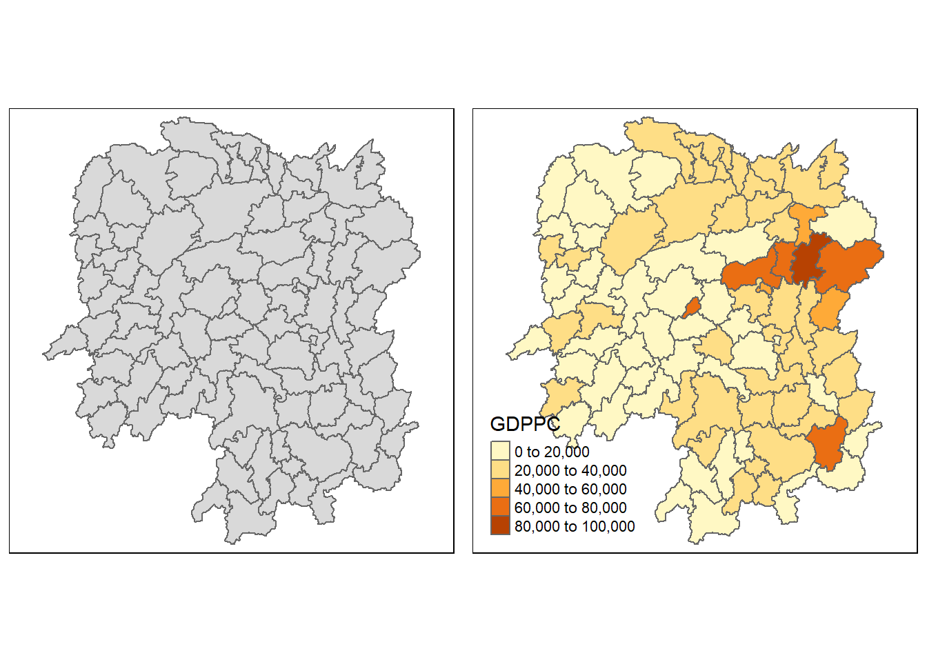
Computing Contiguity Spatial Weights
In this section, the poly2nb() function of the spdep package is used to compute contiguity weight matrices for the study area
- The function builds a neighbour list based on regions with contiguous boundaries, the default of the algorithm uses Queens case, unless explicitly set to false
wm_q = poly2nb(hunan)
summary(wm_q)
Neighbour list object:
Number of regions: 88
Number of nonzero links: 448
Percentage nonzero weights: 5.785124
Average number of links: 5.090909
Link number distribution:
1 2 3 4 5 6 7 8 9 11
2 2 12 16 24 14 11 4 2 1
2 least connected regions:
30 65 with 1 link
1 most connected region:
85 with 11 linkswm_r = poly2nb(hunan, queen = FALSE)
summary(wm_r)Neighbour list object:
Number of regions: 88
Number of nonzero links: 440
Percentage nonzero weights: 5.681818
Average number of links: 5
Link number distribution:
1 2 3 4 5 6 7 8 9 10
2 2 12 20 21 14 11 3 2 1
2 least connected regions:
30 65 with 1 link
1 most connected region:
85 with 10 linksFrom the results, there are 88 regions in Hunan,
Using the Queen’s method, 85 of them has 11 neighbours, while only 2 of them has 1 neighbour
Using the Rook’s method 85 of them has 10 neighbours, while only 2 of them has 1 neighbour
To see neighbours for polygons in the objects, we could reference them like the below for the first polygon:
wm_q[[1]][1] 2 3 4 57 85From the result, we know Polygon 1 has 5 neighbours, the numbers represents the polygon IDs of the respective neighbours stored in the hunan SpatialPolygonsDataFrame class
We can retrieve the county name of polygon ID 1 by using
hunan$County[1][1] "Anxiang"To reveal the names of the 5 neighbours, we can use
hunan$County[c(2,3,4,57,85)][1] "Hanshou" "Jinshi" "Li" "Nan" "Taoyuan"To reveal the GDPPC of these 5 counties, we can use
nb1 = wm_q[[1]]
nb1 = hunan$GDPPC[nb1]
nb1
[1] 20981 34592 24473 21311 22879The result displays the 5 nearest neighbours based on Queen’s method
The complete weight matrix can be displayed by using the str() function
str(wm_q)List of 88
$ : int [1:5] 2 3 4 57 85
$ : int [1:5] 1 57 58 78 85
$ : int [1:4] 1 4 5 85
$ : int [1:4] 1 3 5 6
$ : int [1:4] 3 4 6 85
$ : int [1:5] 4 5 69 75 85
$ : int [1:4] 67 71 74 84
$ : int [1:7] 9 46 47 56 78 80 86
$ : int [1:6] 8 66 68 78 84 86
$ : int [1:8] 16 17 19 20 22 70 72 73
$ : int [1:3] 14 17 72
$ : int [1:5] 13 60 61 63 83
$ : int [1:4] 12 15 60 83
$ : int [1:3] 11 15 17
$ : int [1:4] 13 14 17 83
$ : int [1:5] 10 17 22 72 83
$ : int [1:7] 10 11 14 15 16 72 83
$ : int [1:5] 20 22 23 77 83
$ : int [1:6] 10 20 21 73 74 86
$ : int [1:7] 10 18 19 21 22 23 82
$ : int [1:5] 19 20 35 82 86
$ : int [1:5] 10 16 18 20 83
$ : int [1:7] 18 20 38 41 77 79 82
$ : int [1:5] 25 28 31 32 54
$ : int [1:5] 24 28 31 33 81
$ : int [1:4] 27 33 42 81
$ : int [1:3] 26 29 42
$ : int [1:5] 24 25 33 49 54
$ : int [1:3] 27 37 42
$ : int 33
$ : int [1:8] 24 25 32 36 39 40 56 81
$ : int [1:8] 24 31 50 54 55 56 75 85
$ : int [1:5] 25 26 28 30 81
$ : int [1:3] 36 45 80
$ : int [1:6] 21 41 47 80 82 86
$ : int [1:6] 31 34 40 45 56 80
$ : int [1:4] 29 42 43 44
$ : int [1:4] 23 44 77 79
$ : int [1:5] 31 40 42 43 81
$ : int [1:6] 31 36 39 43 45 79
$ : int [1:6] 23 35 45 79 80 82
$ : int [1:7] 26 27 29 37 39 43 81
$ : int [1:6] 37 39 40 42 44 79
$ : int [1:4] 37 38 43 79
$ : int [1:6] 34 36 40 41 79 80
$ : int [1:3] 8 47 86
$ : int [1:5] 8 35 46 80 86
$ : int [1:5] 50 51 52 53 55
$ : int [1:4] 28 51 52 54
$ : int [1:5] 32 48 52 54 55
$ : int [1:3] 48 49 52
$ : int [1:5] 48 49 50 51 54
$ : int [1:3] 48 55 75
$ : int [1:6] 24 28 32 49 50 52
$ : int [1:5] 32 48 50 53 75
$ : int [1:7] 8 31 32 36 78 80 85
$ : int [1:6] 1 2 58 64 76 85
$ : int [1:5] 2 57 68 76 78
$ : int [1:4] 60 61 87 88
$ : int [1:4] 12 13 59 61
$ : int [1:7] 12 59 60 62 63 77 87
$ : int [1:3] 61 77 87
$ : int [1:4] 12 61 77 83
$ : int [1:2] 57 76
$ : int 76
$ : int [1:5] 9 67 68 76 84
$ : int [1:4] 7 66 76 84
$ : int [1:5] 9 58 66 76 78
$ : int [1:3] 6 75 85
$ : int [1:3] 10 72 73
$ : int [1:3] 7 73 74
$ : int [1:5] 10 11 16 17 70
$ : int [1:5] 10 19 70 71 74
$ : int [1:6] 7 19 71 73 84 86
$ : int [1:6] 6 32 53 55 69 85
$ : int [1:7] 57 58 64 65 66 67 68
$ : int [1:7] 18 23 38 61 62 63 83
$ : int [1:7] 2 8 9 56 58 68 85
$ : int [1:7] 23 38 40 41 43 44 45
$ : int [1:8] 8 34 35 36 41 45 47 56
$ : int [1:6] 25 26 31 33 39 42
$ : int [1:5] 20 21 23 35 41
$ : int [1:9] 12 13 15 16 17 18 22 63 77
$ : int [1:6] 7 9 66 67 74 86
$ : int [1:11] 1 2 3 5 6 32 56 57 69 75 ...
$ : int [1:9] 8 9 19 21 35 46 47 74 84
$ : int [1:4] 59 61 62 88
$ : int [1:2] 59 87
- attr(*, "class")= chr "nb"
- attr(*, "region.id")= chr [1:88] "1" "2" "3" "4" ...
- attr(*, "call")= language poly2nb(pl = hunan)
- attr(*, "type")= chr "queen"
- attr(*, "sym")= logi TRUEVisualizing contiguity weights
In a connectivity graph, each point’s neighbouring points are represented by a line. As the exercise is focused on polygons, points needs to be created before we can build connectivity graphs. Polygon centroids will be the mechanism used for this purpose.
Getting Latitude and Longitude of Polygon Centroids
Before we can create the connectivity graph, we must assign points to each polygon. For this to function, we need the coordinates in a separate data frame. We’ll utilize a mapping function to accomplish this. The mapping function creates a vector of identical length by applying a specified function to each element of a vector. We will use the geometry column of us.bound as our input vector.
st_centroid from the sf package & map_dblfrom the purrr package will be used to accomplish this. We can map the st_centroid function over the geometry column us.bounds to obtain our required values.
The longitude is the first variable in each centroid, this enables us to obtain only the longitude.
The latitude is the second variable in each centroid, this enables us to obtain only the latitude
Using the double bracket notation [[]] and the index, we can access the latitude & longitude values.
longitude = map_dbl(hunan$geometry, ~st_centroid(.x)[[1]]) #longitude index 1
latitude = map_dbl(hunan$geometry, ~st_centroid(.x)[[2]]) #latitude index 2
After getting the longitude and latitudes, we can form the coordinates object named
coordusingcbindUsing the
headfunction, we can inspect the elements ofcoordto verify if they are correctly formattedcoord = cbind(longitude, latitude) head(coord)longitude latitude [1,] 112.1531 29.44362 [2,] 112.0372 28.86489 [3,] 111.8917 29.47107 [4,] 111.7031 29.74499 [5,] 111.6138 29.49258 [6,] 111.0341 29.79863
Plotting Queen contiguity based neighbours map
We can now plot the contiguity graph with our coord object
Using Queen’s method with wm_q
plot(hunan$geometry, border="lightblue")
plot(wm_q, coord, pch = 19, cex = 0.6, add = TRUE, col= "black")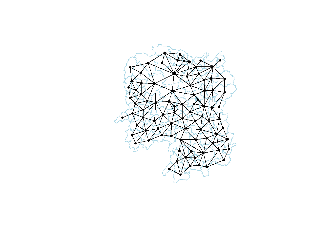
Using Rook’s Method with wm_r
plot(hunan$geometry, border="lightblue")
plot(wm_r, coord, pch = 19, cex = 0.6, add = TRUE, col= "black")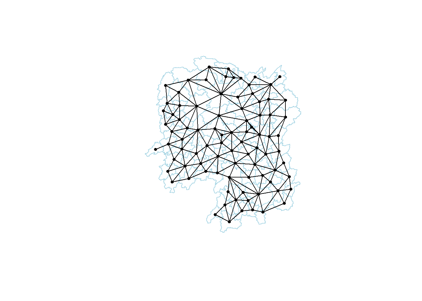
Plotting both Rook’s & Queen’s method
par(mfrow=c(1,2))
plot(hunan$geometry, border="lightblue")
plot(wm_r, coord, pch = 19, cex = 0.6, add = TRUE, col= "black")
plot(hunan$geometry, border="lightblue")
plot(wm_q, coord, pch = 19, cex = 0.6, add = TRUE, col= "black")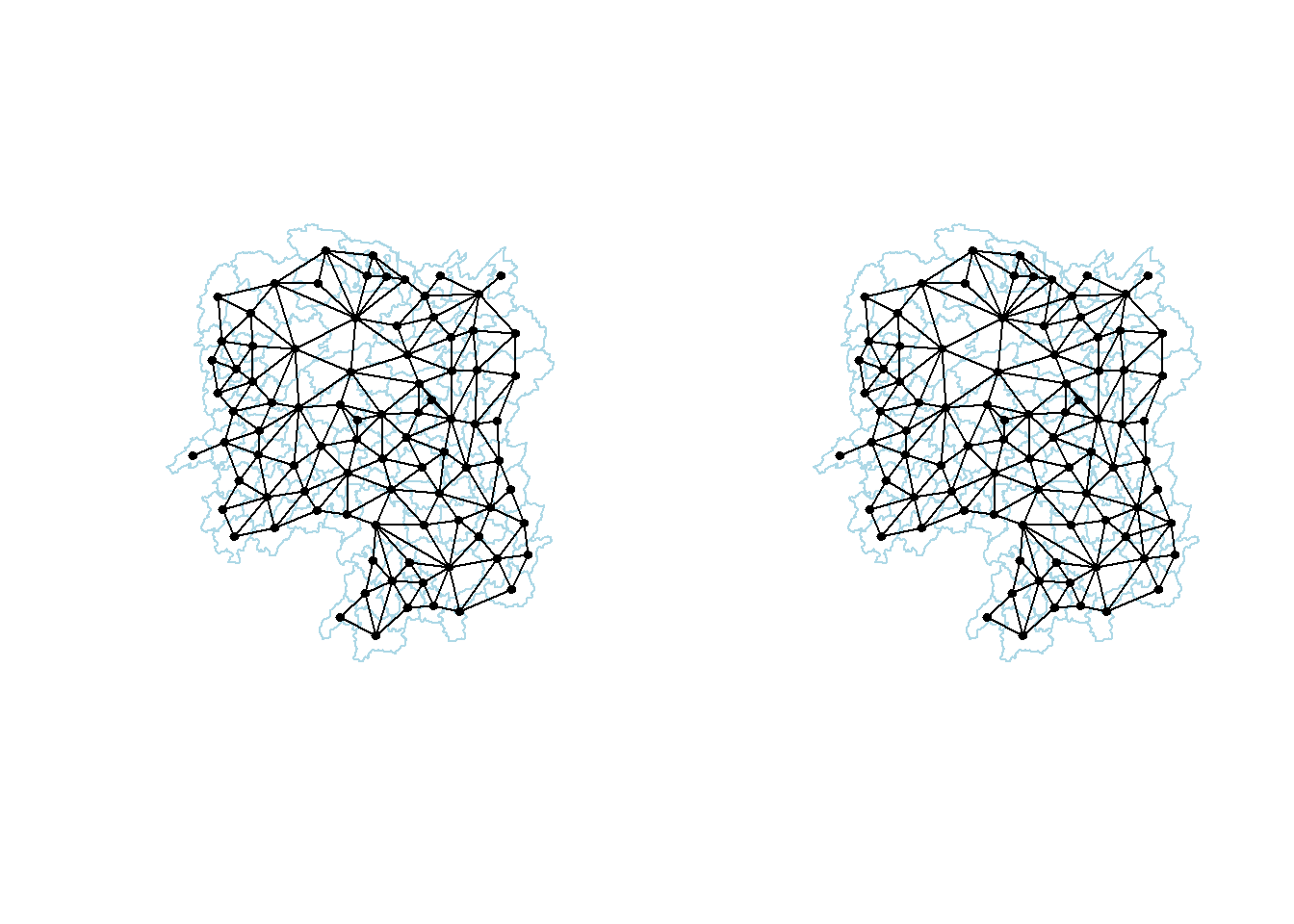
Computing distance based neighbours
With the use of Neighbourhood contiguity by distance - dnearneigh() of spdep package, we can determine the distance based weight matrix.
The function looks for neighbours of regions points by Euclidean distance between the lower (>=) and upper (<=) bound or with the parameter longlat = True by great circle distance in km
Find the lower and upper bounds
Using the k nearest neighbour (knn) algorithm, we can return a matrix with indices of points that belongs to the set of k nearest neighbours of each others by using
knearneigh()of spdepConvert the knn objects into a neighbours list of class nb with a list of integer vectors containing neighbour region number ids by using
knn2nb()Return the length of neighbour relationship edges by using
nbdists()of spdep. The function returns in the units of coordinates if the coordinates are projected, in km otherwise.Remove the list structure of the return objects by using
unlist()
k1 = knn2nb(knearneigh(coord)) #returns a list of nb objects from the result of k nearest neighbours matrix, Step 1 & 2
k1dist = unlist(nbdists(k1, coord, longlat = TRUE)) #return the length of neighbour relationship edges and remove the list structures, Step 3 & 4
summary(k1dist)
Min. 1st Qu. Median Mean 3rd Qu. Max.
24.79 32.57 38.01 39.07 44.52 61.79 From the result, the largest first nearest neighbour is 61.79km, hence by using this as the upper bound, we can be certain that all units will have at least 1 neighbour
Finding the fixed distanced weight matrix
dnearneigh will be used to compute the distance weight matrix
wm_d62 = dnearneigh(coord, 0, 62, longlat = TRUE)
wm_d62
Neighbour list object:
Number of regions: 88
Number of nonzero links: 324
Percentage nonzero weights: 4.183884
Average number of links: 3.681818 The average number of links denotes the number of non zero links divided by the number of regions. In this case, a region has about on average between 3-4 neighbours
Next, we will use str() to display the content of wm_d62 weight matrix.
str(wm_d62)List of 88
$ : int [1:5] 3 4 5 57 64
$ : int [1:4] 57 58 78 85
$ : int [1:4] 1 4 5 57
$ : int [1:3] 1 3 5
$ : int [1:4] 1 3 4 85
$ : int 69
$ : int [1:2] 67 84
$ : int [1:4] 9 46 47 78
$ : int [1:4] 8 46 68 84
$ : int [1:4] 16 22 70 72
$ : int [1:3] 14 17 72
$ : int [1:5] 13 60 61 63 83
$ : int [1:4] 12 15 60 83
$ : int [1:2] 11 17
$ : int 13
$ : int [1:4] 10 17 22 83
$ : int [1:3] 11 14 16
$ : int [1:3] 20 22 63
$ : int [1:5] 20 21 73 74 82
$ : int [1:5] 18 19 21 22 82
$ : int [1:6] 19 20 35 74 82 86
$ : int [1:4] 10 16 18 20
$ : int [1:3] 41 77 82
$ : int [1:4] 25 28 31 54
$ : int [1:4] 24 28 33 81
$ : int [1:4] 27 33 42 81
$ : int [1:2] 26 29
$ : int [1:6] 24 25 33 49 52 54
$ : int [1:2] 27 37
$ : int 33
$ : int [1:2] 24 36
$ : int 50
$ : int [1:5] 25 26 28 30 81
$ : int [1:3] 36 45 80
$ : int [1:6] 21 41 46 47 80 82
$ : int [1:5] 31 34 45 56 80
$ : int [1:2] 29 42
$ : int [1:3] 44 77 79
$ : int [1:4] 40 42 43 81
$ : int [1:3] 39 45 79
$ : int [1:5] 23 35 45 79 82
$ : int [1:5] 26 37 39 43 81
$ : int [1:3] 39 42 44
$ : int [1:2] 38 43
$ : int [1:6] 34 36 40 41 79 80
$ : int [1:5] 8 9 35 47 86
$ : int [1:5] 8 35 46 80 86
$ : int [1:5] 50 51 52 53 55
$ : int [1:4] 28 51 52 54
$ : int [1:6] 32 48 51 52 54 55
$ : int [1:4] 48 49 50 52
$ : int [1:6] 28 48 49 50 51 54
$ : int [1:2] 48 55
$ : int [1:5] 24 28 49 50 52
$ : int [1:4] 48 50 53 75
$ : int 36
$ : int [1:5] 1 2 3 58 64
$ : int [1:5] 2 57 64 66 68
$ : int [1:3] 60 87 88
$ : int [1:4] 12 13 59 61
$ : int [1:5] 12 60 62 63 87
$ : int [1:4] 61 63 77 87
$ : int [1:5] 12 18 61 62 83
$ : int [1:4] 1 57 58 76
$ : int 76
$ : int [1:5] 58 67 68 76 84
$ : int [1:2] 7 66
$ : int [1:4] 9 58 66 84
$ : int [1:2] 6 75
$ : int [1:3] 10 72 73
$ : int [1:2] 73 74
$ : int [1:3] 10 11 70
$ : int [1:4] 19 70 71 74
$ : int [1:5] 19 21 71 73 86
$ : int [1:2] 55 69
$ : int [1:3] 64 65 66
$ : int [1:3] 23 38 62
$ : int [1:2] 2 8
$ : int [1:4] 38 40 41 45
$ : int [1:5] 34 35 36 45 47
$ : int [1:5] 25 26 33 39 42
$ : int [1:6] 19 20 21 23 35 41
$ : int [1:4] 12 13 16 63
$ : int [1:4] 7 9 66 68
$ : int [1:2] 2 5
$ : int [1:4] 21 46 47 74
$ : int [1:4] 59 61 62 88
$ : int [1:2] 59 87
- attr(*, "class")= chr "nb"
- attr(*, "region.id")= chr [1:88] "1" "2" "3" "4" ...
- attr(*, "call")= language dnearneigh(x = coord, d1 = 0, d2 = 62, longlat = TRUE)
- attr(*, "dnn")= num [1:2] 0 62
- attr(*, "bounds")= chr [1:2] "GE" "LE"
- attr(*, "nbtype")= chr "distance"
- attr(*, "sym")= logi TRUEAnother way to display the structure of the weight matrix is to combine table() and card() of spdep.
The
card()function counts the neighboring regions in the neighbours list.table()creates a contingency table of the counts for each combination of factor levels using cross-classifying factors.
cardinality = card(wm_d62)
table(hunan$County, cardinality)
cardinality
1 2 3 4 5 6
Anhua 1 0 0 0 0 0
Anren 0 0 0 1 0 0
Anxiang 0 0 0 0 1 0
Baojing 0 0 0 0 1 0
Chaling 0 0 1 0 0 0
Changning 0 0 1 0 0 0
Changsha 0 0 0 1 0 0
Chengbu 0 1 0 0 0 0
Chenxi 0 0 0 1 0 0
Cili 0 1 0 0 0 0
Dao 0 0 0 1 0 0
Dongan 0 0 1 0 0 0
Dongkou 0 0 0 1 0 0
Fenghuang 0 0 0 1 0 0
Guidong 0 0 1 0 0 0
Guiyang 0 0 0 1 0 0
Guzhang 0 0 0 0 0 1
Hanshou 0 0 0 1 0 0
Hengdong 0 0 0 0 1 0
Hengnan 0 0 0 0 1 0
Hengshan 0 0 0 0 0 1
Hengyang 0 0 0 0 0 1
Hongjiang 0 0 0 0 1 0
Huarong 0 0 0 1 0 0
Huayuan 0 0 0 1 0 0
Huitong 0 0 0 1 0 0
Jiahe 0 0 0 0 1 0
Jianghua 0 0 1 0 0 0
Jiangyong 0 1 0 0 0 0
Jingzhou 0 1 0 0 0 0
Jinshi 0 0 0 1 0 0
Jishou 0 0 0 0 0 1
Lanshan 0 0 0 1 0 0
Leiyang 0 0 0 1 0 0
Lengshuijiang 0 0 1 0 0 0
Li 0 0 1 0 0 0
Lianyuan 0 0 0 0 1 0
Liling 0 1 0 0 0 0
Linli 0 0 0 1 0 0
Linwu 0 0 0 1 0 0
Linxiang 1 0 0 0 0 0
Liuyang 0 1 0 0 0 0
Longhui 0 0 1 0 0 0
Longshan 0 1 0 0 0 0
Luxi 0 0 0 0 1 0
Mayang 0 0 0 0 0 1
Miluo 0 0 0 0 1 0
Nan 0 0 0 0 1 0
Ningxiang 0 0 0 1 0 0
Ningyuan 0 0 0 0 1 0
Pingjiang 0 1 0 0 0 0
Qidong 0 0 1 0 0 0
Qiyang 0 0 1 0 0 0
Rucheng 0 1 0 0 0 0
Sangzhi 0 1 0 0 0 0
Shaodong 0 0 0 0 1 0
Shaoshan 0 0 0 0 1 0
Shaoyang 0 0 0 1 0 0
Shimen 1 0 0 0 0 0
Shuangfeng 0 0 0 0 0 1
Shuangpai 0 0 0 1 0 0
Suining 0 0 0 0 1 0
Taojiang 0 1 0 0 0 0
Taoyuan 0 1 0 0 0 0
Tongdao 0 1 0 0 0 0
Wangcheng 0 0 0 1 0 0
Wugang 0 0 1 0 0 0
Xiangtan 0 0 0 1 0 0
Xiangxiang 0 0 0 0 1 0
Xiangyin 0 0 0 1 0 0
Xinhua 0 0 0 0 1 0
Xinhuang 1 0 0 0 0 0
Xinning 0 1 0 0 0 0
Xinshao 0 0 0 0 0 1
Xintian 0 0 0 0 1 0
Xupu 0 1 0 0 0 0
Yanling 0 0 1 0 0 0
Yizhang 1 0 0 0 0 0
Yongshun 0 0 0 1 0 0
Yongxing 0 0 0 1 0 0
You 0 0 0 1 0 0
Yuanjiang 0 0 0 0 1 0
Yuanling 1 0 0 0 0 0
Yueyang 0 0 1 0 0 0
Zhijiang 0 0 0 0 1 0
Zhongfang 0 0 0 1 0 0
Zhuzhou 0 0 0 0 1 0
Zixing 0 0 1 0 0 0n.comp.nb() finds the number of disjoint connected subgraphs in the graph depicted by nb.obj - a spatial neighbours list object using depth first search
n_comp = n.comp.nb(wm_d62)It returns
nc: number of disjoint connected subgraphs
comp.id: vector with the indices of the disjoint connected subgraphs that the nodes in
nb.objbelong to, in this case the distance weight matrix
n_comp$nc[1] 1#n_comp$comp.id
table(n_comp$comp.id)
 1
88
Plotting fixed distance weight matrix
We can plot the distance weight matrix by using the code below.
plot(hunan$geometry, border="lightblue")
plot(wm_d62, coord, add=TRUE)
plot(k1, coord, add=TRUE, col="red", length = 0.1)
The black lines show the links of neighbours within the cut-off distance of 62km.
The red lines show the links of 1st nearest neighbours
Alternatively, we can plot both of them next to each other with the code below.
par(mfrow=c(1,2))
plot(hunan$geometry, border="lightblue")
plot(wm_d62, coord, add=TRUE)
plot(hunan$geometry, border="lightblue")
plot(k1, coord, add=TRUE, col="red", length = 0.1)
Computing adaptive distance weight matrix
The fixed distance weight matrix has the property that locations with higher densities of habitation (often urban areas) tend to have more neighbours, whereas areas with lower densities (typically rural areas) tend to have fewer neighbours.
By enforcing symmetry or accepting asymmetric neighbours, as shown in the code below, it is possible to control the number of neighbours of each region using the knn algorithm.
knn6 = knn2nb(knearneigh(coord, k=6))Similarly, we can display the content of the matrix by using str()
str(knn6)List of 88
$ : int [1:6] 2 3 4 5 57 64
$ : int [1:6] 1 3 57 58 78 85
$ : int [1:6] 1 2 4 5 57 85
$ : int [1:6] 1 3 5 6 69 85
$ : int [1:6] 1 3 4 6 69 85
$ : int [1:6] 3 4 5 69 75 85
$ : int [1:6] 9 66 67 71 74 84
$ : int [1:6] 9 46 47 78 80 86
$ : int [1:6] 8 46 66 68 84 86
$ : int [1:6] 16 19 22 70 72 73
$ : int [1:6] 10 14 16 17 70 72
$ : int [1:6] 13 15 60 61 63 83
$ : int [1:6] 12 15 60 61 63 83
$ : int [1:6] 11 15 16 17 72 83
$ : int [1:6] 12 13 14 17 60 83
$ : int [1:6] 10 11 17 22 72 83
$ : int [1:6] 10 11 14 16 72 83
$ : int [1:6] 20 22 23 63 77 83
$ : int [1:6] 10 20 21 73 74 82
$ : int [1:6] 18 19 21 22 23 82
$ : int [1:6] 19 20 35 74 82 86
$ : int [1:6] 10 16 18 19 20 83
$ : int [1:6] 18 20 41 77 79 82
$ : int [1:6] 25 28 31 52 54 81
$ : int [1:6] 24 28 31 33 54 81
$ : int [1:6] 25 27 29 33 42 81
$ : int [1:6] 26 29 30 37 42 81
$ : int [1:6] 24 25 33 49 52 54
$ : int [1:6] 26 27 37 42 43 81
$ : int [1:6] 26 27 28 33 49 81
$ : int [1:6] 24 25 36 39 40 54
$ : int [1:6] 24 31 50 54 55 56
$ : int [1:6] 25 26 28 30 49 81
$ : int [1:6] 36 40 41 45 56 80
$ : int [1:6] 21 41 46 47 80 82
$ : int [1:6] 31 34 40 45 56 80
$ : int [1:6] 26 27 29 42 43 44
$ : int [1:6] 23 43 44 62 77 79
$ : int [1:6] 25 40 42 43 44 81
$ : int [1:6] 31 36 39 43 45 79
$ : int [1:6] 23 35 45 79 80 82
$ : int [1:6] 26 27 37 39 43 81
$ : int [1:6] 37 39 40 42 44 79
$ : int [1:6] 37 38 39 42 43 79
$ : int [1:6] 34 36 40 41 79 80
$ : int [1:6] 8 9 35 47 78 86
$ : int [1:6] 8 21 35 46 80 86
$ : int [1:6] 49 50 51 52 53 55
$ : int [1:6] 28 33 48 51 52 54
$ : int [1:6] 32 48 51 52 54 55
$ : int [1:6] 28 48 49 50 52 54
$ : int [1:6] 28 48 49 50 51 54
$ : int [1:6] 48 50 51 52 55 75
$ : int [1:6] 24 28 49 50 51 52
$ : int [1:6] 32 48 50 52 53 75
$ : int [1:6] 32 34 36 78 80 85
$ : int [1:6] 1 2 3 58 64 68
$ : int [1:6] 2 57 64 66 68 78
$ : int [1:6] 12 13 60 61 87 88
$ : int [1:6] 12 13 59 61 63 87
$ : int [1:6] 12 13 60 62 63 87
$ : int [1:6] 12 38 61 63 77 87
$ : int [1:6] 12 18 60 61 62 83
$ : int [1:6] 1 3 57 58 68 76
$ : int [1:6] 58 64 66 67 68 76
$ : int [1:6] 9 58 67 68 76 84
$ : int [1:6] 7 65 66 68 76 84
$ : int [1:6] 9 57 58 66 78 84
$ : int [1:6] 4 5 6 32 75 85
$ : int [1:6] 10 16 19 22 72 73
$ : int [1:6] 7 19 73 74 84 86
$ : int [1:6] 10 11 14 16 17 70
$ : int [1:6] 10 19 21 70 71 74
$ : int [1:6] 19 21 71 73 84 86
$ : int [1:6] 6 32 50 53 55 69
$ : int [1:6] 58 64 65 66 67 68
$ : int [1:6] 18 23 38 61 62 63
$ : int [1:6] 2 8 9 46 58 68
$ : int [1:6] 38 40 41 43 44 45
$ : int [1:6] 34 35 36 41 45 47
$ : int [1:6] 25 26 28 33 39 42
$ : int [1:6] 19 20 21 23 35 41
$ : int [1:6] 12 13 15 16 22 63
$ : int [1:6] 7 9 66 68 71 74
$ : int [1:6] 2 3 4 5 56 69
$ : int [1:6] 8 9 21 46 47 74
$ : int [1:6] 59 60 61 62 63 88
$ : int [1:6] 59 60 61 62 63 87
- attr(*, "region.id")= chr [1:88] "1" "2" "3" "4" ...
- attr(*, "call")= language knearneigh(x = coord, k = 6)
- attr(*, "sym")= logi FALSE
- attr(*, "type")= chr "knn"
- attr(*, "knn-k")= num 6
- attr(*, "class")= chr "nb"Plotting distance based neighbours
plot(hunan$geometry, border="lightblue")
plot(knn6, coord, pch = 19, cex = 0.6, add = TRUE, col = "red")
Weights based on Inverse distance methods
We will need to compute the distances between areas using nbdists() of spdep package
dist = nbdists(wm_q, coord, longlat=TRUE)
ids = lapply(dist, function(x) 1/ (x))
ids
[[1]]
[1] 0.01535405 0.03916350 0.01820896 0.02807922 0.01145113
[[2]]
[1] 0.01535405 0.01764308 0.01925924 0.02323898 0.01719350
[[3]]
[1] 0.03916350 0.02822040 0.03695795 0.01395765
[[4]]
[1] 0.01820896 0.02822040 0.03414741 0.01539065
[[5]]
[1] 0.03695795 0.03414741 0.01524598 0.01618354
[[6]]
[1] 0.015390649 0.015245977 0.021748129 0.011883901 0.009810297
[[7]]
[1] 0.01708612 0.01473997 0.01150924 0.01872915
[[8]]
[1] 0.02022144 0.03453056 0.02529256 0.01036340 0.02284457 0.01500600 0.01515314
[[9]]
[1] 0.02022144 0.01574888 0.02109502 0.01508028 0.02902705 0.01502980
[[10]]
[1] 0.02281552 0.01387777 0.01538326 0.01346650 0.02100510 0.02631658 0.01874863
[8] 0.01500046
[[11]]
[1] 0.01882869 0.02243492 0.02247473
[[12]]
[1] 0.02779227 0.02419652 0.02333385 0.02986130 0.02335429
[[13]]
[1] 0.02779227 0.02650020 0.02670323 0.01714243
[[14]]
[1] 0.01882869 0.01233868 0.02098555
[[15]]
[1] 0.02650020 0.01233868 0.01096284 0.01562226
[[16]]
[1] 0.02281552 0.02466962 0.02765018 0.01476814 0.01671430
[[17]]
[1] 0.01387777 0.02243492 0.02098555 0.01096284 0.02466962 0.01593341 0.01437996
[[18]]
[1] 0.02039779 0.02032767 0.01481665 0.01473691 0.01459380
[[19]]
[1] 0.01538326 0.01926323 0.02668415 0.02140253 0.01613589 0.01412874
[[20]]
[1] 0.01346650 0.02039779 0.01926323 0.01723025 0.02153130 0.01469240 0.02327034
[[21]]
[1] 0.02668415 0.01723025 0.01766299 0.02644986 0.02163800
[[22]]
[1] 0.02100510 0.02765018 0.02032767 0.02153130 0.01489296
[[23]]
[1] 0.01481665 0.01469240 0.01401432 0.02246233 0.01880425 0.01530458 0.01849605
[[24]]
[1] 0.02354598 0.01837201 0.02607264 0.01220154 0.02514180
[[25]]
[1] 0.02354598 0.02188032 0.01577283 0.01949232 0.02947957
[[26]]
[1] 0.02155798 0.01745522 0.02212108 0.02220532
[[27]]
[1] 0.02155798 0.02490625 0.01562326
[[28]]
[1] 0.01837201 0.02188032 0.02229549 0.03076171 0.02039506
[[29]]
[1] 0.02490625 0.01686587 0.01395022
[[30]]
[1] 0.02090587
[[31]]
[1] 0.02607264 0.01577283 0.01219005 0.01724850 0.01229012 0.01609781 0.01139438
[8] 0.01150130
[[32]]
[1] 0.01220154 0.01219005 0.01712515 0.01340413 0.01280928 0.01198216 0.01053374
[8] 0.01065655
[[33]]
[1] 0.01949232 0.01745522 0.02229549 0.02090587 0.01979045
[[34]]
[1] 0.03113041 0.03589551 0.02882915
[[35]]
[1] 0.01766299 0.02185795 0.02616766 0.02111721 0.02108253 0.01509020
[[36]]
[1] 0.01724850 0.03113041 0.01571707 0.01860991 0.02073549 0.01680129
[[37]]
[1] 0.01686587 0.02234793 0.01510990 0.01550676
[[38]]
[1] 0.01401432 0.02407426 0.02276151 0.01719415
[[39]]
[1] 0.01229012 0.02172543 0.01711924 0.02629732 0.01896385
[[40]]
[1] 0.01609781 0.01571707 0.02172543 0.01506473 0.01987922 0.01894207
[[41]]
[1] 0.02246233 0.02185795 0.02205991 0.01912542 0.01601083 0.01742892
[[42]]
[1] 0.02212108 0.01562326 0.01395022 0.02234793 0.01711924 0.01836831 0.01683518
[[43]]
[1] 0.01510990 0.02629732 0.01506473 0.01836831 0.03112027 0.01530782
[[44]]
[1] 0.01550676 0.02407426 0.03112027 0.01486508
[[45]]
[1] 0.03589551 0.01860991 0.01987922 0.02205991 0.02107101 0.01982700
[[46]]
[1] 0.03453056 0.04033752 0.02689769
[[47]]
[1] 0.02529256 0.02616766 0.04033752 0.01949145 0.02181458
[[48]]
[1] 0.02313819 0.03370576 0.02289485 0.01630057 0.01818085
[[49]]
[1] 0.03076171 0.02138091 0.02394529 0.01990000
[[50]]
[1] 0.01712515 0.02313819 0.02551427 0.02051530 0.02187179
[[51]]
[1] 0.03370576 0.02138091 0.02873854
[[52]]
[1] 0.02289485 0.02394529 0.02551427 0.02873854 0.03516672
[[53]]
[1] 0.01630057 0.01979945 0.01253977
[[54]]
[1] 0.02514180 0.02039506 0.01340413 0.01990000 0.02051530 0.03516672
[[55]]
[1] 0.01280928 0.01818085 0.02187179 0.01979945 0.01882298
[[56]]
[1] 0.01036340 0.01139438 0.01198216 0.02073549 0.01214479 0.01362855 0.01341697
[[57]]
[1] 0.028079221 0.017643082 0.031423501 0.029114131 0.013520292 0.009903702
[[58]]
[1] 0.01925924 0.03142350 0.02722997 0.01434859 0.01567192
[[59]]
[1] 0.01696711 0.01265572 0.01667105 0.01785036
[[60]]
[1] 0.02419652 0.02670323 0.01696711 0.02343040
[[61]]
[1] 0.02333385 0.01265572 0.02343040 0.02514093 0.02790764 0.01219751 0.02362452
[[62]]
[1] 0.02514093 0.02002219 0.02110260
[[63]]
[1] 0.02986130 0.02790764 0.01407043 0.01805987
[[64]]
[1] 0.02911413 0.01689892
[[65]]
[1] 0.02471705
[[66]]
[1] 0.01574888 0.01726461 0.03068853 0.01954805 0.01810569
[[67]]
[1] 0.01708612 0.01726461 0.01349843 0.01361172
[[68]]
[1] 0.02109502 0.02722997 0.03068853 0.01406357 0.01546511
[[69]]
[1] 0.02174813 0.01645838 0.01419926
[[70]]
[1] 0.02631658 0.01963168 0.02278487
[[71]]
[1] 0.01473997 0.01838483 0.03197403
[[72]]
[1] 0.01874863 0.02247473 0.01476814 0.01593341 0.01963168
[[73]]
[1] 0.01500046 0.02140253 0.02278487 0.01838483 0.01652709
[[74]]
[1] 0.01150924 0.01613589 0.03197403 0.01652709 0.01342099 0.02864567
[[75]]
[1] 0.011883901 0.010533736 0.012539774 0.018822977 0.016458383 0.008217581
[[76]]
[1] 0.01352029 0.01434859 0.01689892 0.02471705 0.01954805 0.01349843 0.01406357
[[77]]
[1] 0.014736909 0.018804247 0.022761507 0.012197506 0.020022195 0.014070428
[7] 0.008440896
[[78]]
[1] 0.02323898 0.02284457 0.01508028 0.01214479 0.01567192 0.01546511 0.01140779
[[79]]
[1] 0.01530458 0.01719415 0.01894207 0.01912542 0.01530782 0.01486508 0.02107101
[[80]]
[1] 0.01500600 0.02882915 0.02111721 0.01680129 0.01601083 0.01982700 0.01949145
[8] 0.01362855
[[81]]
[1] 0.02947957 0.02220532 0.01150130 0.01979045 0.01896385 0.01683518
[[82]]
[1] 0.02327034 0.02644986 0.01849605 0.02108253 0.01742892
[[83]]
[1] 0.023354289 0.017142433 0.015622258 0.016714303 0.014379961 0.014593799
[7] 0.014892965 0.018059871 0.008440896
[[84]]
[1] 0.01872915 0.02902705 0.01810569 0.01361172 0.01342099 0.01297994
[[85]]
[1] 0.011451133 0.017193502 0.013957649 0.016183544 0.009810297 0.010656545
[7] 0.013416965 0.009903702 0.014199260 0.008217581 0.011407794
[[86]]
[1] 0.01515314 0.01502980 0.01412874 0.02163800 0.01509020 0.02689769 0.02181458
[8] 0.02864567 0.01297994
[[87]]
[1] 0.01667105 0.02362452 0.02110260 0.02058034
[[88]]
[1] 0.01785036 0.02058034Row standardize Weight Matrix
The nb2listw function adds spatial weights for the selected coding scheme to a neighbours list. It’s possible to determine whether a spatial weights object is similar to symmetric and can be transformed in this way to produce real eigenvalues or for Cholesky decomposition.
There are a number of Styles to choose from (Bivand, n.d)
B is the basic binary coding,
W is row standardised (sums over all links to n),
C is globally standardised (sums over all links to n),
U is equal to C divided by the number of neighbours (sums over all links to unity),
S is the variance-stabilizing coding scheme
For this example, we’ll stick with the style=“W” option for simplicity’s but note that other more robust options are available, notably style=“B”, basic binary coding.
rswm_q = nb2listw(wm_q, style="W", zero.policy=TRUE)
rswm_q
Characteristics of weights list object:
Neighbour list object:
Number of regions: 88
Number of nonzero links: 448
Percentage nonzero weights: 5.785124
Average number of links: 5.090909
Weights style: W
Weights constants summary:
n nn S0 S1 S2
W 88 7744 88 37.86334 365.9147Lists of non-neighbours are possible with the zero.policy=TRUE option.
A zero.policy of FALSE would return an error, however this should be used carefully as the user might not be aware of missing neighbors in their dataset.
To view the weight of the first polygon’s 10 neighbour types, we can use the code below
rswm_q$weights[10][[1]]
[1] 0.125 0.125 0.125 0.125 0.125 0.125 0.125 0.125Each neighbor is assigned a 0.125 of the total weight. This means that when R computes the average neighboring income values, each neighbor’s income will be multiplied by 0.125 before being tallied.
Using the same method, we can also derive a row standardized distance weight matrix by using the code below.
rswm_ids <- nb2listw(wm_q, glist=ids, style="B", zero.policy=TRUE)
rswm_ids
Characteristics of weights list object:
Neighbour list object:
Number of regions: 88
Number of nonzero links: 448
Percentage nonzero weights: 5.785124
Average number of links: 5.090909
Weights style: B
Weights constants summary:
n nn S0 S1 S2
B 88 7744 8.786867 0.3776535 3.8137rswm_ids$weights[1][[1]]
[1] 0.01535405 0.03916350 0.01820896 0.02807922 0.01145113summary(unlist(rswm_ids$weights)) Min. 1st Qu. Median Mean 3rd Qu. Max.
0.008218 0.015088 0.018739 0.019614 0.022823 0.040338 Application of Spatial Weight Matrix
In this section, 4 different spatial lagged variables are discussed, they are:
spatial lag with row-standardized weights,
spatial lag as a sum of neighbouring values,
spatial window average,
spatial window sum.
1. Spatial lag with row-standardized weights
First, Compute the average neighbor GDPPC value for each polygon. These values are often referred to as spatially lagged values. We use lag.listw to compute the Spatial lag of a numeric vector
gdppc.lag = lag.listw(rswm_q, hunan$GDPPC)
gdppc.lag
[1] 24847.20 22724.80 24143.25 27737.50 27270.25 21248.80 43747.00 33582.71
[9] 45651.17 32027.62 32671.00 20810.00 25711.50 30672.33 33457.75 31689.20
[17] 20269.00 23901.60 25126.17 21903.43 22718.60 25918.80 20307.00 20023.80
[25] 16576.80 18667.00 14394.67 19848.80 15516.33 20518.00 17572.00 15200.12
[33] 18413.80 14419.33 24094.50 22019.83 12923.50 14756.00 13869.80 12296.67
[41] 15775.17 14382.86 11566.33 13199.50 23412.00 39541.00 36186.60 16559.60
[49] 20772.50 19471.20 19827.33 15466.80 12925.67 18577.17 14943.00 24913.00
[57] 25093.00 24428.80 17003.00 21143.75 20435.00 17131.33 24569.75 23835.50
[65] 26360.00 47383.40 55157.75 37058.00 21546.67 23348.67 42323.67 28938.60
[73] 25880.80 47345.67 18711.33 29087.29 20748.29 35933.71 15439.71 29787.50
[81] 18145.00 21617.00 29203.89 41363.67 22259.09 44939.56 16902.00 16930.00Using the code below, we can append the spatially lag GDPPC values to the Hunan sf data frame.
lag.list = list(hunan$County, gdppc.lag) #lag.listw(rswm_q, hunan$GDPPC)
lag.res = as.data.frame(lag.list)
colnames(lag.res) = c("County", "lag GDPPC")
hunan = left_join(hunan, lag.res)
Joining, by = "County"head(hunan)Simple feature collection with 6 features and 36 fields
Geometry type: POLYGON
Dimension: XY
Bounding box: xmin: 110.4922 ymin: 28.61762 xmax: 112.3013 ymax: 30.12812
Geodetic CRS: WGS 84
NAME_2 ID_3 NAME_3 ENGTYPE_3 Shape_Leng Shape_Area County City
1 Changde 21098 Anxiang County 1.869074 0.10056190 Anxiang Changde
2 Changde 21100 Hanshou County 2.360691 0.19978745 Hanshou Changde
3 Changde 21101 Jinshi County City 1.425620 0.05302413 Jinshi Changde
4 Changde 21102 Li County 3.474325 0.18908121 Li Changde
5 Changde 21103 Linli County 2.289506 0.11450357 Linli Changde
6 Changde 21104 Shimen County 4.171918 0.37194707 Shimen Changde
avg_wage deposite FAI Gov_Rev Gov_Exp GDP GDPPC GIO Loan NIPCR
1 31935 5517.2 3541.0 243.64 1779.5 12482.0 23667 5108.9 2806.9 7693.7
2 32265 7979.0 8665.0 386.13 2062.4 15788.0 20981 13491.0 4550.0 8269.9
3 28692 4581.7 4777.0 373.31 1148.4 8706.9 34592 10935.0 2242.0 8169.9
4 32541 13487.0 16066.0 709.61 2459.5 20322.0 24473 18402.0 6748.0 8377.0
5 32667 564.1 7781.2 336.86 1538.7 10355.0 25554 8214.0 358.0 8143.1
6 33261 8334.4 10531.0 548.33 2178.8 16293.0 27137 17795.0 6026.5 6156.0
Bed Emp EmpR EmpRT Pri_Stu Sec_Stu Household Household_R NOIP Pop_R
1 1931 336.39 270.5 205.9 19.584 17.819 148.1 135.4 53 346.0
2 2560 456.78 388.8 246.7 42.097 33.029 240.2 208.7 95 553.2
3 848 122.78 82.1 61.7 8.723 7.592 81.9 43.7 77 92.4
4 2038 513.44 426.8 227.1 38.975 33.938 268.5 256.0 96 539.7
5 1440 307.36 272.2 100.8 23.286 18.943 129.1 157.2 99 246.6
6 2502 392.05 329.6 193.8 29.245 26.104 190.6 184.7 122 399.2
RSCG Pop_T Agri Service Disp_Inc RORP ROREmp lag GDPPC
1 3957.9 528.3 4524.41 14100 16610 0.6549309 0.8041262 24847.20
2 4460.5 804.6 6545.35 17727 18925 0.6875466 0.8511756 22724.80
3 3683.0 251.8 2562.46 7525 19498 0.3669579 0.6686757 24143.25
4 7110.2 832.5 7562.34 53160 18985 0.6482883 0.8312558 27737.50
5 3604.9 409.3 3583.91 7031 18604 0.6024921 0.8856065 27270.25
6 6490.7 600.5 5266.51 6981 19275 0.6647794 0.8407091 21248.80
geometry
1 POLYGON ((112.0625 29.75523...
2 POLYGON ((112.2288 29.11684...
3 POLYGON ((111.8927 29.6013,...
4 POLYGON ((111.3731 29.94649...
5 POLYGON ((111.6324 29.76288...
6 POLYGON ((110.8825 30.11675...We can plot the GDPPC and spatial lag GDPPC for comparison using the code below
lag_gdppc = tm_shape(hunan) +
        tm_polygons("lag GDPPC")

tmap_arrange(gdppc, lag_gdppc)
2 Spatial lag as a sum of neighboring values
Another way to compute spatial lag as a sum of neigbouring values is by assigning binary weights.
Going back to the neighbours list wm_q, we can apply a function that will assign binary weights by using lapply, and use nb2listw to assign the weights, using the glist parameter to explicitly assign these wieghts
b_weights = lapply(wm_q, function(x) 0*x + 1)
b_weights2 = nb2listw(wm_q, glist = b_weights, style = "B")
b_weights2
Characteristics of weights list object:
Neighbour list object:
Number of regions: 88
Number of nonzero links: 448
Percentage nonzero weights: 5.785124
Average number of links: 5.090909
Weights style: B
Weights constants summary:
n nn S0 S1 S2
B 88 7744 448 896 10224After the weight have been assigned, we can use lag.listw to calculate the lag variable from our weights and GDPPC
lag_sum = list(hunan$County, lag.listw(b_weights2, hunan$GDPPC))
lag.res = as.data.frame(lag_sum)
colnames(lag.res) = c("County", "lag_sum GDPPC")
lag_sum
[[1]]
[1] "Anxiang" "Hanshou" "Jinshi" "Li"
[5] "Linli" "Shimen" "Liuyang" "Ningxiang"
[9] "Wangcheng" "Anren" "Guidong" "Jiahe"
[13] "Linwu" "Rucheng" "Yizhang" "Yongxing"
[17] "Zixing" "Changning" "Hengdong" "Hengnan"
[21] "Hengshan" "Leiyang" "Qidong" "Chenxi"
[25] "Zhongfang" "Huitong" "Jingzhou" "Mayang"
[29] "Tongdao" "Xinhuang" "Xupu" "Yuanling"
[33] "Zhijiang" "Lengshuijiang" "Shuangfeng" "Xinhua"
[37] "Chengbu" "Dongan" "Dongkou" "Longhui"
[41] "Shaodong" "Suining" "Wugang" "Xinning"
[45] "Xinshao" "Shaoshan" "Xiangxiang" "Baojing"
[49] "Fenghuang" "Guzhang" "Huayuan" "Jishou"
[53] "Longshan" "Luxi" "Yongshun" "Anhua"
[57] "Nan" "Yuanjiang" "Jianghua" "Lanshan"
[61] "Ningyuan" "Shuangpai" "Xintian" "Huarong"
[65] "Linxiang" "Miluo" "Pingjiang" "Xiangyin"
[69] "Cili" "Chaling" "Liling" "Yanling"
[73] "You" "Zhuzhou" "Sangzhi" "Yueyang"
[77] "Qiyang" "Taojiang" "Shaoyang" "Lianyuan"
[81] "Hongjiang" "Hengyang" "Guiyang" "Changsha"
[85] "Taoyuan" "Xiangtan" "Dao" "Jiangyong"
[[2]]
[1] 124236 113624 96573 110950 109081 106244 174988 235079 273907 256221
[11] 98013 104050 102846 92017 133831 158446 141883 119508 150757 153324
[21] 113593 129594 142149 100119 82884 74668 43184 99244 46549 20518
[31] 140576 121601 92069 43258 144567 132119 51694 59024 69349 73780
[41] 94651 100680 69398 52798 140472 118623 180933 82798 83090 97356
[51] 59482 77334 38777 111463 74715 174391 150558 122144 68012 84575
[61] 143045 51394 98279 47671 26360 236917 220631 185290 64640 70046
[71] 126971 144693 129404 284074 112268 203611 145238 251536 108078 238300
[81] 108870 108085 262835 248182 244850 404456 67608 33860Examining the result of the lag_sum, the first value of lag_sum is 124236, comparing it with the value in gdppc.lag discussed in Spatial lag with row-standardized weights, the first value was 24847.20.
It can be observed that a weight of 5 has been multiplied. In our earlier discussion, we know that Anxiang has 5 neighbours. Hence, we can conclude that the spatial lag sum method will multiply the result of Spatial lag with row-standardized weights by the number of neighbours in a region.
Using the code below, we can append the spatial lag sum GDPPC values to the Hunan sf data frame.
hunan = left_join(hunan, lag.res)Joining, by = "County"We can plot the GDPPC and spatial lag GDPPC for comparison using the code below
lag_sum_gdppc = tm_shape(hunan) +
        tm_polygons("lag_sum GDPPC")

tmap_arrange(gdppc, lag_sum_gdppc)
3 Spatial window average
The diagonal component is included in the spatial window average, which uses weights that are standardized by row.
Before allocating weights in R, we must return to the neighbours structure and add the diagonal element, the include.self() method from spdep package is used to accomplish that
wm_q_w_diagonal = wm_q
wm_q_w_diagonal = include.self(wm_q_w_diagonal)
wm_q_w_diagonal[[1]]
[1] 1 2 3 4 57 85We will then use nb2listw() to create the weight variable and lag.listw() create the lag variable from the weight structure and GDPPC variable
wm_q_w_diagonal = nb2listw(wm_q_w_diagonal) #compute the weights
lag_w_avg_gdppc = lag.listw(wm_q_w_diagonal, hunan$GDPPC)
lag_w_avg_gdppc
[1] 24650.50 22434.17 26233.00 27084.60 26927.00 22230.17 47621.20 37160.12
[9] 49224.71 29886.89 26627.50 22690.17 25366.40 25825.75 30329.00 32682.83
[17] 25948.62 23987.67 25463.14 21904.38 23127.50 25949.83 20018.75 19524.17
[25] 18955.00 17800.40 15883.00 18831.33 14832.50 17965.00 17159.89 16199.44
[33] 18764.50 26878.75 23188.86 20788.14 12365.20 15985.00 13764.83 11907.43
[41] 17128.14 14593.62 11644.29 12706.00 21712.29 43548.25 35049.00 16226.83
[49] 19294.40 18156.00 19954.75 18145.17 12132.75 18419.29 14050.83 23619.75
[57] 24552.71 24733.67 16762.60 20932.60 19467.75 18334.00 22541.00 26028.00
[65] 29128.50 46569.00 47576.60 36545.50 20838.50 22531.00 42115.50 27619.00
[73] 27611.33 44523.29 18127.43 28746.38 20734.50 33880.62 14716.38 28516.22
[81] 18086.14 21244.50 29568.80 48119.71 22310.75 43151.60 17133.40 17009.33Next, we will convert the lag variable listw object into a data.frame by using as.data.frame()
lag.list.winavg = list(hunan$County, lag.listw(wm_q_w_diagonal, hunan$GDPPC))
lag.list.winavg.res = as.data.frame(lag.list.winavg)
colnames(lag.list.winavg.res) = c("County", "lag_window_avg GDPPC")
Using the code below, we can append the spatial window average GDPPC values to the Hunan sf data frame.
hunan = left_join(hunan, lag.list.winavg.res)Joining, by = "County"We can plot the GDPPC and window average GDPPC for comparison using the code below
win_avg_gdppc = tm_shape(hunan) +
        tm_polygons("lag_window_avg GDPPC")

tmap_arrange(gdppc, win_avg_gdppc)
To compare the values of lag GDPPC and spatial window average kable() of the Knitr package is used
hunan %>% select ("County", "lag GDPPC", "lag_window_avg GDPPC") %>%
kable()| County | lag GDPPC | lag_window_avg GDPPC | geometry |
|---|---|---|---|
| Anxiang | 24847.20 | 24650.50 | POLYGON ((112.0625 29.75523… |
| Hanshou | 22724.80 | 22434.17 | POLYGON ((112.2288 29.11684… |
| Jinshi | 24143.25 | 26233.00 | POLYGON ((111.8927 29.6013,… |
| Li | 27737.50 | 27084.60 | POLYGON ((111.3731 29.94649… |
| Linli | 27270.25 | 26927.00 | POLYGON ((111.6324 29.76288… |
| Shimen | 21248.80 | 22230.17 | POLYGON ((110.8825 30.11675… |
| Liuyang | 43747.00 | 47621.20 | POLYGON ((113.9905 28.5682,… |
| Ningxiang | 33582.71 | 37160.12 | POLYGON ((112.7181 28.38299… |
| Wangcheng | 45651.17 | 49224.71 | POLYGON ((112.7914 28.52688… |
| Anren | 32027.62 | 29886.89 | POLYGON ((113.1757 26.82734… |
| Guidong | 32671.00 | 26627.50 | POLYGON ((114.1799 26.20117… |
| Jiahe | 20810.00 | 22690.17 | POLYGON ((112.4425 25.74358… |
| Linwu | 25711.50 | 25366.40 | POLYGON ((112.5914 25.55143… |
| Rucheng | 30672.33 | 25825.75 | POLYGON ((113.6759 25.87578… |
| Yizhang | 33457.75 | 30329.00 | POLYGON ((113.2621 25.68394… |
| Yongxing | 31689.20 | 32682.83 | POLYGON ((113.3169 26.41843… |
| Zixing | 20269.00 | 25948.62 | POLYGON ((113.7311 26.16259… |
| Changning | 23901.60 | 23987.67 | POLYGON ((112.6144 26.60198… |
| Hengdong | 25126.17 | 25463.14 | POLYGON ((113.1056 27.21007… |
| Hengnan | 21903.43 | 21904.38 | POLYGON ((112.7599 26.98149… |
| Hengshan | 22718.60 | 23127.50 | POLYGON ((112.607 27.4689, … |
| Leiyang | 25918.80 | 25949.83 | POLYGON ((112.9996 26.69276… |
| Qidong | 20307.00 | 20018.75 | POLYGON ((111.7818 27.0383,… |
| Chenxi | 20023.80 | 19524.17 | POLYGON ((110.2624 28.21778… |
| Zhongfang | 16576.80 | 18955.00 | POLYGON ((109.9431 27.72858… |
| Huitong | 18667.00 | 17800.40 | POLYGON ((109.9419 27.10512… |
| Jingzhou | 14394.67 | 15883.00 | POLYGON ((109.8186 26.75842… |
| Mayang | 19848.80 | 18831.33 | POLYGON ((109.795 27.98008,… |
| Tongdao | 15516.33 | 14832.50 | POLYGON ((109.9294 26.46561… |
| Xinhuang | 20518.00 | 17965.00 | POLYGON ((109.227 27.43733,… |
| Xupu | 17572.00 | 17159.89 | POLYGON ((110.7189 28.30485… |
| Yuanling | 15200.12 | 16199.44 | POLYGON ((110.9652 28.99895… |
| Zhijiang | 18413.80 | 18764.50 | POLYGON ((109.8818 27.60661… |
| Lengshuijiang | 14419.33 | 26878.75 | POLYGON ((111.5307 27.81472… |
| Shuangfeng | 24094.50 | 23188.86 | POLYGON ((112.263 27.70421,… |
| Xinhua | 22019.83 | 20788.14 | POLYGON ((111.3345 28.19642… |
| Chengbu | 12923.50 | 12365.20 | POLYGON ((110.4455 26.69317… |
| Dongan | 14756.00 | 15985.00 | POLYGON ((111.4531 26.86812… |
| Dongkou | 13869.80 | 13764.83 | POLYGON ((110.6622 27.37305… |
| Longhui | 12296.67 | 11907.43 | POLYGON ((110.985 27.65983,… |
| Shaodong | 15775.17 | 17128.14 | POLYGON ((111.9054 27.40254… |
| Suining | 14382.86 | 14593.62 | POLYGON ((110.389 27.10006,… |
| Wugang | 11566.33 | 11644.29 | POLYGON ((110.9878 27.03345… |
| Xinning | 13199.50 | 12706.00 | POLYGON ((111.0736 26.84627… |
| Xinshao | 23412.00 | 21712.29 | POLYGON ((111.6013 27.58275… |
| Shaoshan | 39541.00 | 43548.25 | POLYGON ((112.5391 27.97742… |
| Xiangxiang | 36186.60 | 35049.00 | POLYGON ((112.4549 28.05783… |
| Baojing | 16559.60 | 16226.83 | POLYGON ((109.7015 28.82844… |
| Fenghuang | 20772.50 | 19294.40 | POLYGON ((109.5239 28.19206… |
| Guzhang | 19471.20 | 18156.00 | POLYGON ((109.8968 28.74034… |
| Huayuan | 19827.33 | 19954.75 | POLYGON ((109.5647 28.61712… |
| Jishou | 15466.80 | 18145.17 | POLYGON ((109.8375 28.4696,… |
| Longshan | 12925.67 | 12132.75 | POLYGON ((109.6337 29.62521… |
| Luxi | 18577.17 | 18419.29 | POLYGON ((110.1067 28.41835… |
| Yongshun | 14943.00 | 14050.83 | POLYGON ((110.0003 29.29499… |
| Anhua | 24913.00 | 23619.75 | POLYGON ((111.6034 28.63716… |
| Nan | 25093.00 | 24552.71 | POLYGON ((112.3232 29.46074… |
| Yuanjiang | 24428.80 | 24733.67 | POLYGON ((112.4391 29.1791,… |
| Jianghua | 17003.00 | 16762.60 | POLYGON ((111.6461 25.29661… |
| Lanshan | 21143.75 | 20932.60 | POLYGON ((112.2286 25.61123… |
| Ningyuan | 20435.00 | 19467.75 | POLYGON ((112.0715 26.09892… |
| Shuangpai | 17131.33 | 18334.00 | POLYGON ((111.8864 26.11957… |
| Xintian | 24569.75 | 22541.00 | POLYGON ((112.2578 26.0796,… |
| Huarong | 23835.50 | 26028.00 | POLYGON ((112.9242 29.69134… |
| Linxiang | 26360.00 | 29128.50 | POLYGON ((113.5502 29.67418… |
| Miluo | 47383.40 | 46569.00 | POLYGON ((112.9902 29.02139… |
| Pingjiang | 55157.75 | 47576.60 | POLYGON ((113.8436 29.06152… |
| Xiangyin | 37058.00 | 36545.50 | POLYGON ((112.9173 28.98264… |
| Cili | 21546.67 | 20838.50 | POLYGON ((110.8822 29.69017… |
| Chaling | 23348.67 | 22531.00 | POLYGON ((113.7666 27.10573… |
| Liling | 42323.67 | 42115.50 | POLYGON ((113.5673 27.94346… |
| Yanling | 28938.60 | 27619.00 | POLYGON ((113.9292 26.6154,… |
| You | 25880.80 | 27611.33 | POLYGON ((113.5879 27.41324… |
| Zhuzhou | 47345.67 | 44523.29 | POLYGON ((113.2493 28.02411… |
| Sangzhi | 18711.33 | 18127.43 | POLYGON ((110.556 29.40543,… |
| Yueyang | 29087.29 | 28746.38 | POLYGON ((113.343 29.61064,… |
| Qiyang | 20748.29 | 20734.50 | POLYGON ((111.5563 26.81318… |
| Taojiang | 35933.71 | 33880.62 | POLYGON ((112.0508 28.67265… |
| Shaoyang | 15439.71 | 14716.38 | POLYGON ((111.5013 27.30207… |
| Lianyuan | 29787.50 | 28516.22 | POLYGON ((111.6789 28.02946… |
| Hongjiang | 18145.00 | 18086.14 | POLYGON ((110.1441 27.47513… |
| Hengyang | 21617.00 | 21244.50 | POLYGON ((112.7144 26.98613… |
| Guiyang | 29203.89 | 29568.80 | POLYGON ((113.0811 26.04963… |
| Changsha | 41363.67 | 48119.71 | POLYGON ((112.9421 28.03722… |
| Taoyuan | 22259.09 | 22310.75 | POLYGON ((112.0612 29.32855… |
| Xiangtan | 44939.56 | 43151.60 | POLYGON ((113.0426 27.8942,… |
| Dao | 16902.00 | 17133.40 | POLYGON ((111.498 25.81679,… |
| Jiangyong | 16930.00 | 17009.33 | POLYGON ((111.3659 25.39472… |
4 Spatial window sum
The spatial window sum is the counter part of the window average, but without using row-standardized weights.
To do this we assign binary weights to the neighbour structure that includes the diagonal element, similar to the one done in Spatial lag as a sum of neighboring values
wm_q_w_diagonal = wm_q
wm_q_w_diagonal = include.self(wm_q_w_diagonal)
b_weights_winsum = lapply(wm_q_w_diagonal, function(x) 0*x + 1)
b_weights_winsum[1]
[[1]]
[1] 1 1 1 1 1 1Similar to the one done in Spatial lag as a sum of neighboring values, we use nb2listw() and glist parameter to explicitly assign weight values.
b_weights_winsum2 = nb2listw(wm_q_w_diagonal, glist=b_weights_winsum, style="B")
b_weights_winsum2
Characteristics of weights list object:
Neighbour list object:
Number of regions: 88
Number of nonzero links: 536
Percentage nonzero weights: 6.921488
Average number of links: 6.090909
Weights style: B
Weights constants summary:
n nn S0 S1 S2
B 88 7744 536 1072 14160With the new weight structure, the new lag variable can be derived by using lag.listw()
w_sum_gdppc = list(hunan$County, lag.listw(b_weights_winsum2, hunan$GDPPC))
w_sum_gdppc
[[1]]
[1] "Anxiang" "Hanshou" "Jinshi" "Li"
[5] "Linli" "Shimen" "Liuyang" "Ningxiang"
[9] "Wangcheng" "Anren" "Guidong" "Jiahe"
[13] "Linwu" "Rucheng" "Yizhang" "Yongxing"
[17] "Zixing" "Changning" "Hengdong" "Hengnan"
[21] "Hengshan" "Leiyang" "Qidong" "Chenxi"
[25] "Zhongfang" "Huitong" "Jingzhou" "Mayang"
[29] "Tongdao" "Xinhuang" "Xupu" "Yuanling"
[33] "Zhijiang" "Lengshuijiang" "Shuangfeng" "Xinhua"
[37] "Chengbu" "Dongan" "Dongkou" "Longhui"
[41] "Shaodong" "Suining" "Wugang" "Xinning"
[45] "Xinshao" "Shaoshan" "Xiangxiang" "Baojing"
[49] "Fenghuang" "Guzhang" "Huayuan" "Jishou"
[53] "Longshan" "Luxi" "Yongshun" "Anhua"
[57] "Nan" "Yuanjiang" "Jianghua" "Lanshan"
[61] "Ningyuan" "Shuangpai" "Xintian" "Huarong"
[65] "Linxiang" "Miluo" "Pingjiang" "Xiangyin"
[69] "Cili" "Chaling" "Liling" "Yanling"
[73] "You" "Zhuzhou" "Sangzhi" "Yueyang"
[77] "Qiyang" "Taojiang" "Shaoyang" "Lianyuan"
[81] "Hongjiang" "Hengyang" "Guiyang" "Changsha"
[85] "Taoyuan" "Xiangtan" "Dao" "Jiangyong"
[[2]]
[1] 147903 134605 131165 135423 134635 133381 238106 297281 344573 268982
[11] 106510 136141 126832 103303 151645 196097 207589 143926 178242 175235
[21] 138765 155699 160150 117145 113730 89002 63532 112988 59330 35930
[31] 154439 145795 112587 107515 162322 145517 61826 79925 82589 83352
[41] 119897 116749 81510 63530 151986 174193 210294 97361 96472 108936
[51] 79819 108871 48531 128935 84305 188958 171869 148402 83813 104663
[61] 155742 73336 112705 78084 58257 279414 237883 219273 83354 90124
[71] 168462 165714 165668 311663 126892 229971 165876 271045 117731 256646
[81] 126603 127467 295688 336838 267729 431516 85667 51028Next, we will convert the lag variable listw object into a data.frame by using as.data.frame()
w_sum_gdppc.res = as.data.frame(w_sum_gdppc)
colnames(w_sum_gdppc.res) = c("County", "w_sum GDPPC")
Using the code below, we can append the spatial window sum GDPPC values to the Hunan sf data frame.
hunan = left_join(hunan, w_sum_gdppc.res)Joining, by = "County"To compare the values of lag GDPPC and spatial window average kable() of the Knitr package is used
hunan %>% select ("County", "lag_sum GDPPC", "w_sum GDPPC") %>%
kable()| County | lag_sum GDPPC | w_sum GDPPC | geometry |
|---|---|---|---|
| Anxiang | 124236 | 147903 | POLYGON ((112.0625 29.75523… |
| Hanshou | 113624 | 134605 | POLYGON ((112.2288 29.11684… |
| Jinshi | 96573 | 131165 | POLYGON ((111.8927 29.6013,… |
| Li | 110950 | 135423 | POLYGON ((111.3731 29.94649… |
| Linli | 109081 | 134635 | POLYGON ((111.6324 29.76288… |
| Shimen | 106244 | 133381 | POLYGON ((110.8825 30.11675… |
| Liuyang | 174988 | 238106 | POLYGON ((113.9905 28.5682,… |
| Ningxiang | 235079 | 297281 | POLYGON ((112.7181 28.38299… |
| Wangcheng | 273907 | 344573 | POLYGON ((112.7914 28.52688… |
| Anren | 256221 | 268982 | POLYGON ((113.1757 26.82734… |
| Guidong | 98013 | 106510 | POLYGON ((114.1799 26.20117… |
| Jiahe | 104050 | 136141 | POLYGON ((112.4425 25.74358… |
| Linwu | 102846 | 126832 | POLYGON ((112.5914 25.55143… |
| Rucheng | 92017 | 103303 | POLYGON ((113.6759 25.87578… |
| Yizhang | 133831 | 151645 | POLYGON ((113.2621 25.68394… |
| Yongxing | 158446 | 196097 | POLYGON ((113.3169 26.41843… |
| Zixing | 141883 | 207589 | POLYGON ((113.7311 26.16259… |
| Changning | 119508 | 143926 | POLYGON ((112.6144 26.60198… |
| Hengdong | 150757 | 178242 | POLYGON ((113.1056 27.21007… |
| Hengnan | 153324 | 175235 | POLYGON ((112.7599 26.98149… |
| Hengshan | 113593 | 138765 | POLYGON ((112.607 27.4689, … |
| Leiyang | 129594 | 155699 | POLYGON ((112.9996 26.69276… |
| Qidong | 142149 | 160150 | POLYGON ((111.7818 27.0383,… |
| Chenxi | 100119 | 117145 | POLYGON ((110.2624 28.21778… |
| Zhongfang | 82884 | 113730 | POLYGON ((109.9431 27.72858… |
| Huitong | 74668 | 89002 | POLYGON ((109.9419 27.10512… |
| Jingzhou | 43184 | 63532 | POLYGON ((109.8186 26.75842… |
| Mayang | 99244 | 112988 | POLYGON ((109.795 27.98008,… |
| Tongdao | 46549 | 59330 | POLYGON ((109.9294 26.46561… |
| Xinhuang | 20518 | 35930 | POLYGON ((109.227 27.43733,… |
| Xupu | 140576 | 154439 | POLYGON ((110.7189 28.30485… |
| Yuanling | 121601 | 145795 | POLYGON ((110.9652 28.99895… |
| Zhijiang | 92069 | 112587 | POLYGON ((109.8818 27.60661… |
| Lengshuijiang | 43258 | 107515 | POLYGON ((111.5307 27.81472… |
| Shuangfeng | 144567 | 162322 | POLYGON ((112.263 27.70421,… |
| Xinhua | 132119 | 145517 | POLYGON ((111.3345 28.19642… |
| Chengbu | 51694 | 61826 | POLYGON ((110.4455 26.69317… |
| Dongan | 59024 | 79925 | POLYGON ((111.4531 26.86812… |
| Dongkou | 69349 | 82589 | POLYGON ((110.6622 27.37305… |
| Longhui | 73780 | 83352 | POLYGON ((110.985 27.65983,… |
| Shaodong | 94651 | 119897 | POLYGON ((111.9054 27.40254… |
| Suining | 100680 | 116749 | POLYGON ((110.389 27.10006,… |
| Wugang | 69398 | 81510 | POLYGON ((110.9878 27.03345… |
| Xinning | 52798 | 63530 | POLYGON ((111.0736 26.84627… |
| Xinshao | 140472 | 151986 | POLYGON ((111.6013 27.58275… |
| Shaoshan | 118623 | 174193 | POLYGON ((112.5391 27.97742… |
| Xiangxiang | 180933 | 210294 | POLYGON ((112.4549 28.05783… |
| Baojing | 82798 | 97361 | POLYGON ((109.7015 28.82844… |
| Fenghuang | 83090 | 96472 | POLYGON ((109.5239 28.19206… |
| Guzhang | 97356 | 108936 | POLYGON ((109.8968 28.74034… |
| Huayuan | 59482 | 79819 | POLYGON ((109.5647 28.61712… |
| Jishou | 77334 | 108871 | POLYGON ((109.8375 28.4696,… |
| Longshan | 38777 | 48531 | POLYGON ((109.6337 29.62521… |
| Luxi | 111463 | 128935 | POLYGON ((110.1067 28.41835… |
| Yongshun | 74715 | 84305 | POLYGON ((110.0003 29.29499… |
| Anhua | 174391 | 188958 | POLYGON ((111.6034 28.63716… |
| Nan | 150558 | 171869 | POLYGON ((112.3232 29.46074… |
| Yuanjiang | 122144 | 148402 | POLYGON ((112.4391 29.1791,… |
| Jianghua | 68012 | 83813 | POLYGON ((111.6461 25.29661… |
| Lanshan | 84575 | 104663 | POLYGON ((112.2286 25.61123… |
| Ningyuan | 143045 | 155742 | POLYGON ((112.0715 26.09892… |
| Shuangpai | 51394 | 73336 | POLYGON ((111.8864 26.11957… |
| Xintian | 98279 | 112705 | POLYGON ((112.2578 26.0796,… |
| Huarong | 47671 | 78084 | POLYGON ((112.9242 29.69134… |
| Linxiang | 26360 | 58257 | POLYGON ((113.5502 29.67418… |
| Miluo | 236917 | 279414 | POLYGON ((112.9902 29.02139… |
| Pingjiang | 220631 | 237883 | POLYGON ((113.8436 29.06152… |
| Xiangyin | 185290 | 219273 | POLYGON ((112.9173 28.98264… |
| Cili | 64640 | 83354 | POLYGON ((110.8822 29.69017… |
| Chaling | 70046 | 90124 | POLYGON ((113.7666 27.10573… |
| Liling | 126971 | 168462 | POLYGON ((113.5673 27.94346… |
| Yanling | 144693 | 165714 | POLYGON ((113.9292 26.6154,… |
| You | 129404 | 165668 | POLYGON ((113.5879 27.41324… |
| Zhuzhou | 284074 | 311663 | POLYGON ((113.2493 28.02411… |
| Sangzhi | 112268 | 126892 | POLYGON ((110.556 29.40543,… |
| Yueyang | 203611 | 229971 | POLYGON ((113.343 29.61064,… |
| Qiyang | 145238 | 165876 | POLYGON ((111.5563 26.81318… |
| Taojiang | 251536 | 271045 | POLYGON ((112.0508 28.67265… |
| Shaoyang | 108078 | 117731 | POLYGON ((111.5013 27.30207… |
| Lianyuan | 238300 | 256646 | POLYGON ((111.6789 28.02946… |
| Hongjiang | 108870 | 126603 | POLYGON ((110.1441 27.47513… |
| Hengyang | 108085 | 127467 | POLYGON ((112.7144 26.98613… |
| Guiyang | 262835 | 295688 | POLYGON ((113.0811 26.04963… |
| Changsha | 248182 | 336838 | POLYGON ((112.9421 28.03722… |
| Taoyuan | 244850 | 267729 | POLYGON ((112.0612 29.32855… |
| Xiangtan | 404456 | 431516 | POLYGON ((113.0426 27.8942,… |
| Dao | 67608 | 85667 | POLYGON ((111.498 25.81679,… |
| Jiangyong | 33860 | 51028 | POLYGON ((111.3659 25.39472… |
We can plot the GDPPC and window sum GDPPC for comparison using the code below
win_sum_gdppc = tm_shape(hunan) +
        tm_polygons("w_sum GDPPC")

tmap_arrange(gdppc, win_sum_gdppc)
Reference
Kam T.S (2022), R for Geospatial Data Science and Analytics, Chapter 3 Spatial Weights and Applications
https://r4gdsa.netlify.app/chap03.html
Bivand R (n.d) Spatial weights for neighbours lists
https://r-spatial.github.io/spdep/reference/nb2listw.html